PS-2020a / part14

- Standard -​

- Standard -​

C Measuring the Accuracy With Which a​ Display System Matches the Grayscale​ Standard Display Function (Informative)​

C.1 General Considerations Regarding Conformance and Metrics​

TodemonstrateconformancewiththeGrayscaleStandardDisplayFunctionisamuchmorecomplextaskthan,forexample,validating​ the responses of a totally digital system to DICOM messages.​

Display systems ultimately produce analog output, either directly as Luminances or indirectly as optical densities. For some Display​ Systems,thisanalogoutputcanbeaffectedbyvariousimperfectionsinadditiontowhateverimperfectionsexistintheDisplaySystem's​ Display Function that is to be validated. For example, there may be spatial non-uniformities in the final presented image (e.g., arising​ fromfilm,printing,orprocessingnon-uniformitiesinthecaseofahardcopyprinter)thataremeasurablebutareatlowspatialfrequencies​ that do not ordinarily pose an image quality problem in diagnostic radiology.​

It is worth noting that CRTs and light-boxes also introduce their own spatial non-uniformities. These non-uniformities are outside the​ scope of the Grayscale Standard Display Function and the measurement procedures described here. But because of them, even a​ test image that is perfectly presented in terms of the Grayscale Standard Display Function will be less than perfectly perceived on a​ real CRT or a real light-box.​

Furthermore, the question "How close (to the Grayscale Standard Display Function) is close enough?" is currently unanswered, since​ the answer depends on psychophysical studies not yet done to determine what difference in Display Function is "just noticeable"​ when two nearly identical image presentations (e.g., two nearly identical films placed on equivalent side-by-side light-boxes) are​ presented to an observer.​

Furthermore, the evaluation of a given Display System could be based either on visual tests (e.g., assessing the perceived contrast​ ofmanylow-contrasttargetsinoneormoretestimages)orbyquantitativeanalysisbasedonmeasureddataobtainedfrominstruments​ (e.g., photometers or densitometers).​

Even the quantitative approach could be addressed in different ways. One could, for example, simply superimpose plots of measured​ and theoretical analog output (i.e., Luminance or optical density) vs. P-Value, perhaps along with "error bars" indicating the expected​ uncertainty (non-repeatable variations) in the measured output. As a mathematically more elegant alternative, all the measured data​ points could be used as input to a statistical mathematical analysis that could attempt to determine the underlying Display Function​ of the Display System, yielding one or more quantitative values (metrics) that define how well the Display System conforms with the​ Grayscale Standard Display Function.​

In what follows in this and the following annexes, an example of the latter type of metric analysis is used, in which measured data is​ analyzed using a "FIT" test that is intended to validate the shape of the Characteristic Curve and a "LUM" test that is intended to show​ thedegreeofscatterfromtheidealGrayscaleStandardDisplayFunction.Thisapproachhasbeenapplied,forexample,toquantitatively​ demonstrate how improvements were successfully made to the Display Function of certain Display Systems.​

Before proceeding with the description of the methodology of this specific metric approach, it should be noted that it is offered as one​ possible approach, not necessarily as the most appropriate approach for evaluating all Display Systems. In particular, the following​ notes should be considered before selecting or interpreting results from any particular metric approach.​

1.​There may be practical issues that limit the number of P-Values that can be meaningfully used in the analysis. For example, it​ may be practical to measure all 256 possible Luminances from a fixed position on the screen of an 8-bit video monitor, but it may​ be impractical to meaningfully measure all 4096 densities theoretically printable by a 12-bit film printer. One reason for the im-​ practicalityisthelimitedaccuracyofdensitometers(orevenfilmdigitizers).Asecondreasonisthatthefilmdensitymeasurements,​ unliketheCRTphotometermeasurements,areobtainedfromdifferentlocationsonthedisplayarea,soanyspatialnon-uniformity​ that is present in the film affects the hardcopy measurement. Current hardcopy printers and densitometers both have absolute​ optical density accuracy limitations that are significantly worse than the change that would be caused by a change in just the​ least significant bit of a 12-bit P-Value. In general, selecting a larger number of P-Values allows, in principle, more localized ab-​ errations from the Grayscale Standard Display Function to be "caught", but the signal-to-noise ratio (or significance) of each of​ these will be decreased.​

- Standard -​

2.​If the measurement data for a particular Display System has significant "noise" (as indicated by limited repeatability in the data​ when multiple sets of measurements are taken), it may be desirable to apply a statistical analysis technique that goes beyond​ the "FIT" and "LUM" metric by explicitly utilizing the known standard deviations in the input data, along with the data itself, to​ preventthefittingtechniquefromover-reactingtonoise.See,forexample,thesection"GeneralLinearLeastSquares"inReference​ C1andthechapter"Least-SquaresFittoaPolynomial"inReferenceC2.Ifmeasurementnoiseisnotexplicitlytakenintoaccount​ in the analysis, the metric's returned root-mean-square error of the data points relative to the fit could be misleadingly high, since​ it would include the combined effect of errors due to incorrectness in the Display Function and errors due to measurement noise.​

3.​If possible, the sensitivity and specificity of the metric being considered should be checked against visual tests. For example, a​ digitaltestpatternwithmanylow-contraststepsatmanyambientLuminancescouldbeprintedona"laboratorystandard"Grayscale​ Standard Display Function printer and also printed on a printer being evaluated. The resultant films could then be placed side-​ by-side on light-boxes for comparison by a human observer. A good metric technique should detect as sensitively and repeatably​ as the human observer the existence of deviations (of any shape) from the Grayscale Standard Display Function. For example,​ if a Display System has a Characteristic Curve that, for even a very short interval of DDL values, is too contrasty, too flat, or​ (worse yet) non-monotonic, the metric should be able to detect and respond to that anomaly as strongly as the human observer​ does.​

4.​Finally, in addition to the experimentally encountered non-repeatabilities in the data from a Display System, there may be reason​ to consider additional possible causes of variations. For example, varying the ordering of P-Values in a test pattern (temporally​ for CRTs, spatially for printers) might affect the results. For printers, switching to different media might affect the results. A higher​ confidence can be placed in the results obtained from any metric if the results are stable in the presence of any or all such​ changes.​

C.2 Methodology​

Step (1)​

The Characteristic Curve of the test Display System should be determined with as many measurements as practical (see Section D.1,​ Section D.2, and Section D.3). Using the Grayscale Standard Display Function, the fractional number of JNDs are calculated for each​ Luminance interval between equally spaced P-Value steps. The JNDs/Luminance interval may be calculated directly, or iteratively.​ For example, if only a few JNDs belong to every Luminance interval, a linear interpolation may be performed. After transformation of​ the grayscale response of the Display System, the Luminance Levels for every P-Value are Li and the corresponding Standard Lu-​ minance Levels are Lj; dj specifies the JNDs /Luminance-Interval on the Grayscale Standard Display Function for the given number​ of P-Values. Then, the JNDs/Luminance interval for the transformed Display Function are​

Additionally, an iterative method can be used to calculate the number of JNDs per Luminance interval, requiring only the Grayscale​ Standard Display Function that defines a JND step in Luminance given a Luminance value. This is done by simply counting the​ number of complete JND steps in the Luminance interval, and then the remaining fractional step. Start at the Luminance low end of​ the interval, and calculate from the Grayscale Standard Display Function the Luminance step required for one JND step. Then con-​ tinue stepping from the low Luminance value to the high Luminance value in single JND steps, until the Luminance value of the upper​ end of the Luminance Range is passed. Calculate the fraction portion of one JND that this last step represents. the total number of​ completed integer JND steps plus the fractional portion of the last uncompleted step is the fractional number of JND steps in the Lu-​ minance interval.​

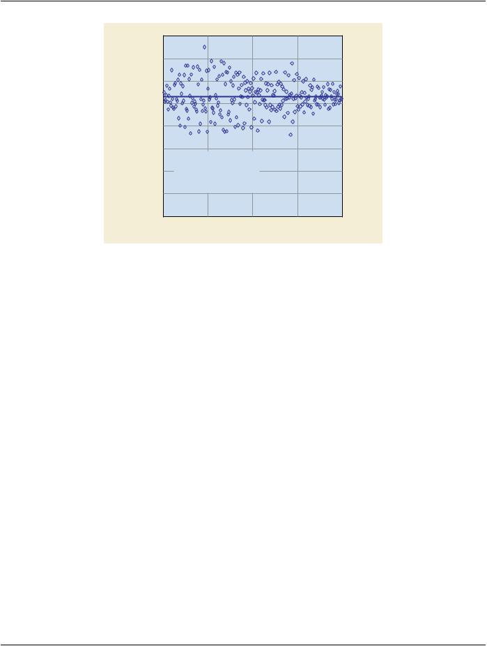
Plot the number of JNDs per Luminance interval (vertical axis) versus the index of the Luminance interval (horizontal axis). This curve​ is referred to as the Luminance intervals vs JNDscurve. An example of a plot of Luminance intervals vs JNDs is shown in figure C-1.​ The plot is matched very well by a horizontal line when a linear regression is applied.​

- Standard -​

I, INDEX OF LUMINANCE INTERVAL

Figure C-1. Illustration for the LUM and FIT conformance measures​

The JNDs/Luminance interval data are evaluated by two statistical measures [C4]. The first assesses the global match of the test​ Display Function with the Grayscale Standard Display Function. The second measure locally analyses the approximation of the​ Grayscale Standard Display Function to the test Display Function.​

Step (2)​

Two related measures of a regression analysis are applied after normal multiple linear regression assumptions are verified for the​ data [C3].The first measure, named the FITtest, attempts to match the Luminance-Intervals-vs-JNDs curve of the test Luminance​ distribution with different order polynomial fits. The Grayscale Standard Display Function is characterized by exactly one JND per​ LuminanceintervalovertheentireLuminanceRange.Therefore,ideally,thedataofJNDs/LuminanceintervalsvsindexoftheLuminance​ interval are best fit by a horizontal line of a constant number of JNDs/Luminance interval, indicating that both the local and global​ means of JNDs/Luminance interval are constant over the given Luminance Range. If the curve is better matched by a higher-order​ curve, the distribution is not closely approximating the Grayscale Standard Display Function. The regression analysis should test​ comparisons through third-order curves.​

The second measure, the Luminance uniformity metric (LUM), analyzes whether the size of Luminance steps are uniform in percep-​ tual size (i.e., JNDs) across the Luminance Range. This is measured by the Root Mean Square Error (RMSE) of the curve fit by a​ horizontal line of the JNDs/Luminance interval. The smaller the RMSE of the JNDs/Luminance interval, the more closely the test​ Display Function approximates the Grayscale Standard Display Function on a microscopic scale.​

Both the FIT and LUM measures can be conveniently calculated on standard statistical packages.​

Assuming the test Luminance distribution passes the FIT test, then the measure of quality of the distribution is determined by the​ single quantitative measurement (LUM) of the standard deviation of the JNDs/Luminance interval from their mean. Clinical practice​ is expected to determine the tolerances for the FIT and LUM values.​

An important factor in reaching a close approximation of a test Display Function to the Grayscale Standard Display Function is the​ number of discrete output levels of the Display System. For instance, the LUM measure can be improved by using only a subset of​ the available DDLs while maintaining the full available output digitization resolution at the cost of decreasing contrast resolution.​

While the LUM is influenced by the choice of the number of discrete output gray levels in the Grayscale Standard Display Function,​ the appropriate number of output levels is determined by the clinical application, including possible gray scale image processing that​ may occur independently of the Grayscale Standard Display Function standardization. Thus, PS3.14 does not prescribe a certain​ number of gray levels of output. However, in general, the larger the number of distinguishable gray levels available, the higher the​ possible image quality because the contrast resolution is increased. It is recommended that the number of necessary output driving​

- Standard -​

levelsforthetransformedDisplayFunctionbedeterminedpriortostandardizationoftheDisplaySystem(basedonclinicalapplications​ of the Display System), so that this information can be used when calculating the transformation in order to avoid using gray scale​ distributions with fewer output levels than needed.​

C.3 References​

[C1] Press, William H, et al., Numerical Recipes in C, Cambridge University Press, 1988, Section "General Linear Least Squares"​

[C2]Bevington,PhillipR.,DataReductionandErrorAnalysisforthePhysicalSciences,McGraw-Hill,1969,thechapter"Least-Squares​ Fit to a Polynomial" .​

[C3]KleinbaumDG,KupperLL,MullerKE,AppliedRegressionAnalysisandOtherMultivariableMethods,DuxburyPress,2ndEdition,​ pp 45-49, 1987.​

[C4] Hemminger, B., Muller, K., "Performance Metric for evaluating conformance of medical image displays with the ACR/NEMA​ display function standard", SPIE Medical Imaging 1997, editor Yongmin Kim, vol 3031-25, 1997.​

- Standard -​

D Illustrations for Achieving Conformance​ withtheGrayscaleStandardDisplayFunction​ (Informative)​

The following sections illustrate how conformance with the Grayscale Standard Display Function may be achieved for emissive (soft-​ copy) Display Systems as well as systems producing image presentations (hard-copies) on transmissive and reflective media. Each​ sectioncontainsfoursub-sectionson1)aprocedureformeasuringthesystemCharacteristicCurve,2)theapplicationoftheGrayscale​ Standard Display Function to the Luminance Range of the Display System, 3) the implementation of the Grayscale Standard Display​ Function, and 4) the application of the conformance metrics as proposed in Annex C.​

It is emphasized that there are different ways to configure a Display System or to change its performance so that it conforms to the​ GrayscaleStandardDisplayFunction.Infact,conceivably,aDisplaySystemmaycalibrateitselfautomaticallytomaintainconformance​ with the Standard. Hence, the following three illustrations are truly only examples.​

Luminance of any Display System, hard-copy or softcopy, may be measured with a photometer. The photometer should have the​ following characteristics:​

•​be accurate to within 3% or less of the absolute Luminance level across its full range of operation;​

•​have a relative accuracy of at least two times the least significant digit at any Luminance level in its range of operation;​

•​maintain this accuracy at Luminance levels that are one-tenth of the minimum measured Luminance of the Display System;​

•​have an acceptance angle that is small enough to incorporate only the measurement field without overlapping the surrounding​ background.​

Note​

The photometer may be of the type that attaches directly to the display face (with a suction cup) or of the type that is held​ away from the display face. If of the latter type, the photometer should be well baffled to exclude extraneous light sources,​ including light from the background area of the test pattern.​

For a film Display System the photometer may be appropriately used to measure the background Illuminance and the Luminance of​ the light-box on which the film will be displayed. The Luminance characteristics of the film Display System may be measured directly​ with the photometer or indirectly using measured optical density of the film and the values for the measured background Illuminance​ and the light-box Luminance.​

D.1 Emissive Display Systems​

D.1.1 Measuring the System Characteristic Curve​

BeforethecharacteristicLuminanceresponseoftheemissiveDisplaySystemismeasured,itisallowedtowarmupasrecommended​ by the manufacturer and is adjusted such that it conforms to the manufacturer's performance specifications. In particular, adjustment​ procedures for setting the black and white levels of the display should be obtained from the Display System manufacturer. The goal​ is to maximize the dynamic Luminance Range of the display without introducing artifacts, resulting in the highest possible number of​ Just-Noticeable Differences (JNDs).​

Note​

A simple test that the system is set up properly can be performed by viewing the 5% and 95% squares in the SMPTE pattern.​ The perceived contrast between the 5% square and its 0% surrounding should be equal to the perceived contrast between​ the 95% square and a white square.​

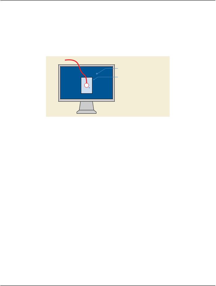
Measurement of the Characteristic Curve of the Display System may be accomplished using a test pattern (Figure D.1-1) consisting​ of:​

- Standard -​

•​a square measurement field comprising 10% of the total number of pixels displayed by the system positioned in the center of the​ display;​

•​a full-screen uniform background of 20% of maximum Luminance surrounding the target.​

Note​

Withameasurementfieldof10%ofthetotalnumberofdisplayedpixelsandasurroundingsetto20%ofmaximumLuminance,​ internal light scatter in the monitor causes the Luminance Range to be typically comparable to that found in radiographs,​ such as a thorax radiograph, when displayed on the CRT monitor.​

Background - 20% of maximum luminance

Target - 10% of the total number of pixels, positioned in the center of the screen

Photometer - suction cup type shown

Figure D.1-1. The test pattern will be a variable intensity square in the center of a low Luminance​ background area.​

Note​

1.​For example, on a 5-megapixel Display System with a matrix of 2048 by 2560 pixels, the target would be a square with​ 724 pixels on each side.​

2.​Ideally, the test pattern should fill the entire screen. Under certain windowed operating environments, it may be difficult​ to eliminate certain user-interface objects from the display, in particular, menu bars at the top of the screen. In this case,​ the background should fill as much of the screen as possible.​

The Characteristic Curve of the Display System may be determined by​

•​turning off all ambient lighting (necessary only when a suction cup photometer is used or when a handheld photometer casts a​ shadow on the display screen);​

•​displaying the above test pattern;​

•​setting the DDL for the measurement field to a sequence of different values, starting with 0 and increasing at each step until the​ maximum DDL is reached;​

•​using a photometer to measure and record the Luminance of the measurement field at each command value.​

As discussed in Annex C, the number and distribution of DDLs at which measurements are taken must be sufficient to accurately​ model the Characteristic Curve of the Display System over the entire Luminance Range.​

Note​

1.​If a handheld photometer is used, it should be placed at a distance from the display screen so that Luminance is​ measured in the center of the measurement field, without overlapping the surrounding background. This distance can​ be calculated using the acceptance angle specification provided by the photometer manufacturer.​

2.​The exact number and distribution of DDLs should be based both on the characteristics of the Display System and on​ the mathematical technique used to interpolate the Characteristic Curve of the system. It is recommended that at least​ 64 different command values be used in the procedure.​

- Standard -​

3.​Successive Luminance measurements should be spaced in time such that the Display System always reaches a steady​ state. It may be particularly important to allow the system to settle before taking the initial measurement at DDL 0.​

As stated in the normative section, the effect of ambient light on the apparent Characteristic Curve must always be included when​ configuring a Display System to conform with the Grayscale Standard Display Function.​

If a handheld photometer that does not cast a shadow on the display screen is used to measure the Characteristic Curve, then the​ Luminance produced by the display plus the effect of ambient light may be measured simultaneously.​

When a suction cup photometer is used to take the Luminance measurements or when a handheld photometer casts a shadow on​ the display screen, all ambient lighting should be turned off while measuring the Characteristic Curve. The effect of ambient light is​ determined separately: The Display System is turned off, the ambient light is turned on, and the Luminance produced by scattering​ ofambientlightatthedisplayscreenismeasuredbyplacingthephotometeratadistancefromthedisplayscreensothatitsacceptance​ angle includes a major portion of the screen and that the measurement is not affected by direct illumination from areas outside the​ displayscreen.TheLuminancerelatedtoambientlightisaddedtothepreviouslymeasuredLuminancelevelsproducedbytheDisplay​ System to determine the effective Characteristic Curve of the system.​

Note​

Changes in ambient lighting conditions may require recalibration of the display subsystem in order to maintain conformance​ to this Standard.​

In the following, an example for measurements and transformation of a Display Function is presented. The Display System for this​ example is a CRT monitor with display controller. It is assumed that the display controller allows a transformation of the DDLs with​ 8-bit input precision and 10-bit output precision.​

The Luminance is measured with a photometer with a narrow (1°) acceptance angle. The ambient light level was adjusted as low as​ possible. No localized highlights were visible.​

1.​The maximum Luminance was measured when setting the DDL for the measurement field to the value that yielded the highest​ Luminance and the DDL of the surrounding to the middle DDL range. From this measurement, the Luminance - 20% of the​ maximum Luminance - for the surrounding of the measurement field was calculated.​

2.​The ambient light was turned off. With the photometer centered on the measurement field of the test pattern of Figure D.1-1, the​ Luminance was measured when varying the input level Dm in increments of 1 from 0 to 255. The transformation operator of the​ hypothetical display controller linearly mapped 8 bits on the input to 10 bits on the output. The measured data represent the​ Characteristic Curve L = F(Dm) for the given operating conditions and this test pattern.​

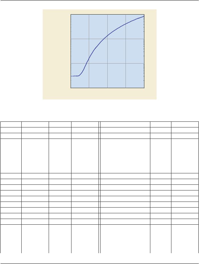
3.​Next,theCRTwasturnedoffandtheambientlightturnedon.ThephotometerwasplacedonthecenteraxisoftheCRTsufficiently​ far away so that it did not cast a shadow on the CRT face and its aperture intercepted light scattered from a major portion of the​ CRT face. The measured Luminance of 0.3 cd/m2produced by the ambient light on the CRT face was added to the measured​ Luminance values of the Characteristic Curve without ambient light. The result is listed in Table D.1-1 and plotted in Figure D.1-​ 2.​

- Standard -​

DIGITAL DRIVING LEVEL

Figure D.1-2. Measured Characteristic Curve with Ambient Light of an emissive Display System​

Table D.1-1. Measured Characteristic Curve plus Ambient Light​

- Standard -​