1.5.1. General assumptions. Components of the poynting vector

Let us carry out our consideration under the paraxial approximation. In contrast to the traditional approach [95], we will consider not only time-averaged Poynting vector, but also instantaneous Poynting vector. There are the reasons for such consideration:

1. Temporal averaging has a sense for optical waves alone, because of too rapid temporal changes of a field. What is concerned to the electromagnetic waves of radio frequency domain, the oscillation period is often comparable with the relaxation time of the physical system. In this case, influence of the wave on such system is determined by the behavior of non-averaged Poynting vector or, at least, by the behavior of this vector averaged over much smaller interval of time .Similarly, the concept of the Nye dsclination is the fundamental notion for radio waves, which loses its fruitfulness in optics [80,81].

2. Let us not also that consideration of the temporal behavior of the components supplies additional information for more deep understanding of the processes leading to the formation of the averaged Poynting vector.

Let the -axis be coinciding with the prevailing direction of the wave energy propagation. The orientation of the -axes is not relevant and may be specified arbitrary.

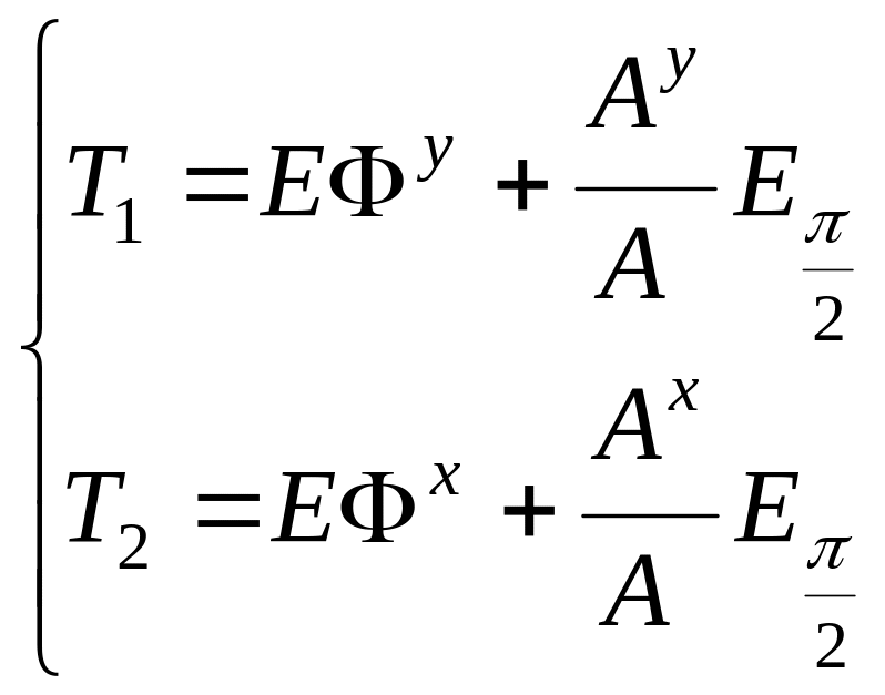
The following relations for the Poynting vector’s components are valid under paraxial approximation (see Appendix 1.3):

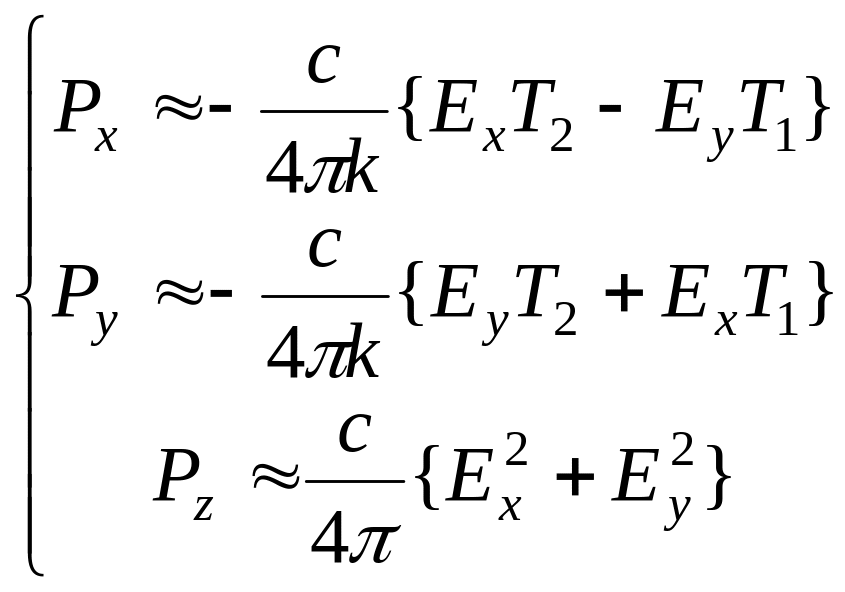, (1.153)

where

, (1.154)

and

, (1.155)

are the amplitudes and phases of the components, respectively, are their derivatives, and .

It follows from Eqs. (1.153)-(1.155) that under paraxial approximation the Poynting vector’s components can be represented as the functions determined by the -components alone. Just these equations and their versions will be the basic ones in our further analysis.

1.5.2. Singularities of the poynting vector in scalar fields

Let us specify the notion of a scalar field. As a rule, one considers a uniformly polarized field as the scalar one, irrespective of the type of polarization [8]. Hereinafter, we reduce the notion of a scalar field to the linearly polarized one, while the behavior of the Poynting vector for elliptically polarized field can be very sophisticated. In part, elliptically polarized wave possesses s-called spin angular momentum [95,100].

1.5.2.1. Instantaneous singularities of a scalar field

The basic scalar equations for the wave polarized along -axis (the choice of the axis is not relevant) have the form:

, (1.156)

, (1.157)

. (1.158)

It follows from Eqs. (1.156)-(1.158) that singularities of the Poynting vector arise in two cases: (i) all three components vanish simultaneously; this case corresponds to appearance of the disclination; (ii) only transversal component vanishes; this case corresponds to simultaneous vanishing of and .

Really, in this case, orientation of the transversal component of the Poynting vector (its azimuth ) is undeterminate.

Thus, appearance of the defect of the Poynting vector for simultaneously vanishing three components requires more precise definition of the notion of disclination of a scalar field. In contrast to the vector field, where disclinations are the lines moving within 3D space (or the corresponding points in any cross-section of the field), disclinations in scalar field degenerate into zero surfaces (or the corresponding closed lines in any cross-section of the field). So, in contrast to the vector field, where disclinations are the “point-like” singularities, in a scalar field they are moving “edge” singularities. Moreover, point disclinations do not exist in a scalar field, what follows from the field’s continuity and from the fact that amplitude of a linearly polarized wave vanishes at each point of the field twice per period of oscillations.

Such behavior of the field is illustrated by the behavior of the transversal component of the Poynting vector in the vicinity of an isotropic vortex in Figure 1.56.

a b c d

Figure 1.56. Rotation of the edge disclination in the vicinity of an isotropic vortex.

a – intensity distribution for an isotropic vortex; b-d – instantaneous distributions of the modulus of the transversal Poynting vector component for different moments, which determines the position of disclination. Temporal step between the figures b-c is 1/12 of oscillation period.

a b c

Figure 1.57. Instantaneous orientation of the transverse component of the Poynting vector for different moments. Temporal step between the figures is 1/16 of the oscillation period.

It can be seen that the transverse component rotates around the vortex center with the doubled frequency of oscillations, and the direction of rotation is determined by the sign of the topological charge of a vortex.

I nstantaneous orientation of the Poynting vector’s component for different instants represented in Figure 1.57 is described by the following relation:

, (1.159)

where is the topological charge of a vortex.

I

a b

Figure 1.58. Circulation of the averaged Poynting vector in vicinity the vortex center.

t follows from Eq. (1.159) and Figure 1.57 that the azimuth of the Poynting vector for some instant does not depend on . It is changed by jump under the crossing of disclination. Thus, the well-known circulation of the averaged Poynting vector in the vicinity of the vortex center, cf. Ref. 96, results from the averaging of similarly oriented vectors.

It is seen from this figure that the azimuth of the averaged component of the Poynting vector has a singularity at the vortex center, which is kind of the “center” [101]. Both cases, (a) and (b) are associated with the positive Poincare index, . That is why one must introduce the additional parameter, viz. chirality , for comprehensive characteristics of such singularity of the Poynting vector. Let us assume that the field propagates in the direction toward to the observer. Let the positive chirality, (cf. Figure 1.58(b)) being corresponding to the clockwise vector circulation, and the negative chirality, (cf. Figure 1.58(a)) being corresponding to the counterclockwise vector circulation. Hereinafter, we will referred to such singularities of the azimuth of the Poynting vector (as well as similar to them) as the vortex singularities.

The situation is much more complicated for the scalar field of general form, but behavior of the Poynting vector is the same as in the case of isotropic vortex. Temporal behavior of the transversal component for the area of a random scalar field is illustrated in the signs of their topological charges. Disclinations rotating in opposite directions and corresponding to the adjacent vortices converge at the saddle points of a phase, cf. Figures 1.59(b),(c),(d), and again diverge in the direction orthogonal to the direction of convergence, see Figure 1.59(a). The direction of motion of the disclinations is indicated by white arrows.

a b c d

Figure 1.59. Temporal behavior of the transverse component modulus of a random scalar field. The direction of moving of the disclication indicated by white arrows. Temporal step between the figures is ¼ of oscillation period.

The second kind of the instantaneous defects arising in a scalar field is constituted by the defects of transversal component of the Poynting vector corresponding to its zero magnitude and non-zero magnitude of -component. Such singularities are point-like. Possible realizations of the point-like singularities can be reduced to the structures shown in Figure 1.60.

In contrast to the vortex singularities, the averaged angular momentum of the field over the spatial coordinates and short temporal interval vanishes in the nearest vicinity of such singularity. Hereinafter we will refer to the singularities of this kind as “passive singularities”.

Let us assign the name “positive passive singularities” for the singularities, which are presented in the Fig.60a (by analogy with the fluxes behavior in the

v icinity of the positive electric charge). Singularities presented in Fig.6b,c we will call, hereinafter, as “negative” and “saddle passive singularities”, respectively.

Specific behavior of the transversal component of the Poynting vector at the areas corresponding to all kinds of point-lke singularities resulting from a computer simulation is illustrated in Figure 1.61.

I

Figure 1.60. Instantaneous “passive” singularities. (a) – negative singularity; (b),(c) – positive singularities.

t is seen from Figs. 1.60 and 1.61 that the passive singularities can be characterized by both the positive (cf. Figures 1.60(a),(b) and 1.61(a),(c)) and negative (cf. Figures 1.60(c) and 1.61(b)) Poincare index.

T

a b c

Figure 1.61 Behavior of the transversal component of the Poynting vector at the areas corresponding to all kinds of point-like singularities resulting from a computer simulation.

he adjacent passive singularities with the opposite signs of the Poincare index are connected by the current lines of the transversal component of the Poynting vector into singular nets. For that, the saddle character of a saddle singularity provides the topological connection between the singularities with positive indices. That is why such singularities are born and annihilate by pairs (with plus- and minus- indices) without arising of additional singularities.

The motion of such singularities is governed by some regularities. In part, analysis of Eqs. (1.156)-(1.158) (impossibility of simultaneous vanishing of and ) leads to the conclusion that the point-like passive singularities inavoidably pass through all stationary points of a phase and intensity.