3. Integration of the differential equation of fluid equilibrium

Let us consider the integration of the differential equation of fluid equilibrium in the form (A.3') or (A.6) for three specific cases, which were discussed in Chapters II and III, namely, the principal case of equilibrium of a fluid under the action of gravity and the two cases of relative rest.

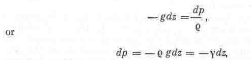
1. Let gravity be the only body force acting on a fluid. Directing the z axis vertically up, we have

X=0; Y=0; Z = —g.

Substituting into Eq. (A.3’), we obtain

The integration constant can be found from the free-surface conditions where, at z = z₀, p = p₀ (see Fig. 6). Consequently,

We have thus arrived at Eq. (2.2), which was developed in another way in Sec. 6.

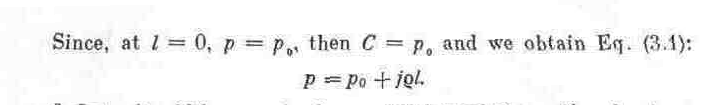
2. Let a liquid be contained in a vessel moving with uniform acceleration in a straight line, i.e., the case of relative rest of a liquid discussed in Sec. 11. Here Eq. (A.6) is more convenient, the direction of l being taken parallel to the resultant body force j (see Fig. 19). We have

262

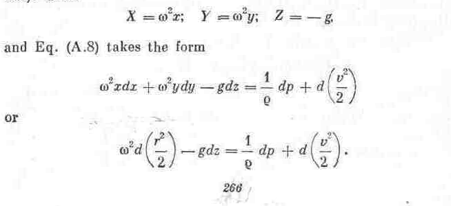
3. Let a liquid be contained in a vessel revolving uniformly about its vertical axis with an angular velocity ω, i. e., the case of relative rest examined in Sec. 12. Placing the origin of the coordinate system in the center of the bottom and directing the x axis straight up, we have

Substituting these values into the equilibrium equation (A.3'), we obtain

Taking into account that

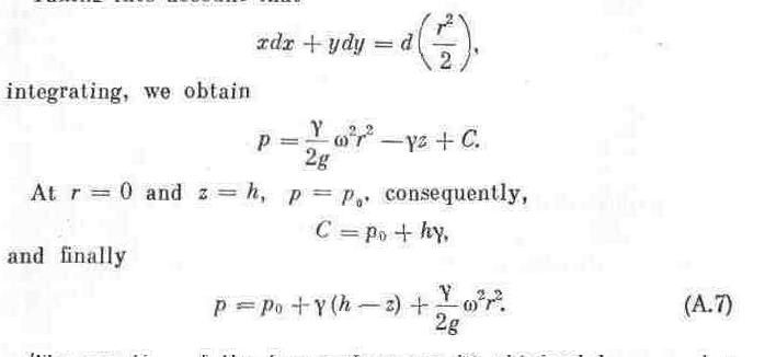
The equation of the tree surface can be obtained by assuming p = p₀ in Eq. (A.7). Canceling out and performing the necessary transformations, we obtain

which fully agrees with Eq. (3.2) obtained before.

263

If in the above discourse gravity is neglected (Z = 0) and the integration constant is determined from the condition that, at r = r₀, p=p_0, we obtain Eq. (3.3):

4. Integration of the differential equations of fluid flow

Considering the case of steady flow, multiply each of the equations (A.I) by the respective projections of the elementary displacement, which are

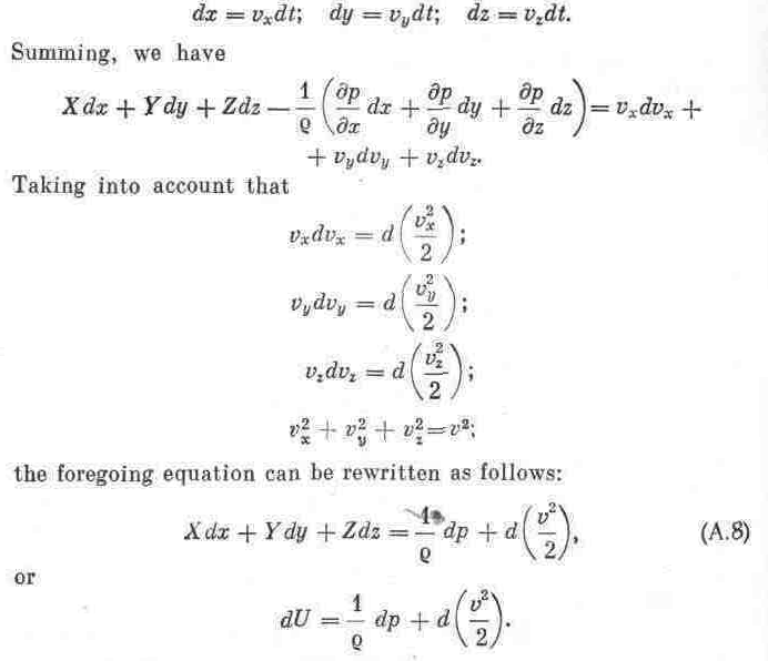
Let us integrate this equation for the principal case of ideal fluid flow, when gravity is the only body force acting on the fluid, and for the two cases of relative motion.

1. Directing the z axis vertically up, in the first case we have

X=0; У=0; Z = -g.

264

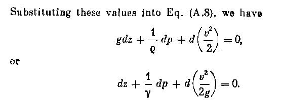
Since for an incompressible fluid γ = const, the foregoing equation can be written in the form

This equation means that the increment of the sum of the three terms in the parentheses in a displacement along a streamline (or pathline) is zero. We conclude from this that the trinomial is a constant along the streamline and, consequently, along the whole of a differential stream tube, i. e.,

This is Bernoulli's equation for a stream tube of an ideal fluid, which we developed in Sec. 15.

Written between two cross-sections of the stream tube, the equa­tion takes the familiar form (4.12):

2. Let a liquid be flowing along a channel which is in turn moving through space with a uniform acceleration a (Fig. 104). Acting on all the fluid particles will be a unit body force , numerically equal to the acceleration but oppositely directed. Denoting the components of this force by

Integrating and carrying out the basic transformations, we have

If this equation is written between two cross-sections of a stream tube with the coordinates of their centres of gravity at х₁, y_l, z_l and x₂, y₂, z₂ it takes the form

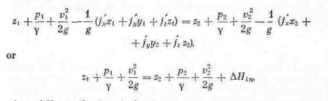
where ΔH_in is the inertia head

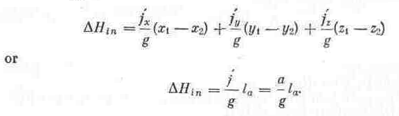
Here l_a is the length of the projection of the portion of the stream tube (or channel) under consideration on the direction of the acceleration a, i. e., the distance between the two points (x₁, y_l, z₁) and (x₂, y₂, z₂). The same results were obtained in Sec. 40.

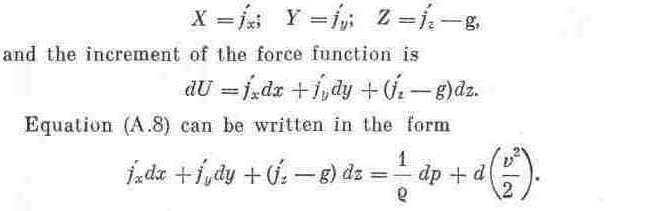
3. Let a liquid be flowing through a channel, which is revolving uniformly about a vertical axis with an angular velocity ω (Fig. 105). Then

After integration and the necessary transformations,

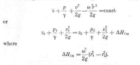
We have thus arrived at the equation (10.3) developed in Sec. 40.

Thus, all the basic equilibrium and flow equations for an ideal fluid which we originally obtained by the specific physical phenomena investigating can be developed very nicely by integrating Euler's general differential equations.

267