Differential equations of ideal fluid flow and their integration

1. Differential equations of ideal fluid flow

Let us show that the fundamental equations of hydrostatics and Bernoulli's equation for the cases discussed before can be developed by integrating of the ideal fluid flow differential equations. We shall develop these equations and then integrate them for the main special cases of equilibrium and motion.

In a steady stream of an ideal fluid take an arbitrary point M whose coordinates are x, y, z (Fig. 178). In some differential time interval dt a fluid particle will move from point M to point M'. The displacement is dl, and its projections on the coordinate axes are dx, dy, dz. The segment dl is thus a pathline element, which, in the case of steady motion, coincides with the streamline.

Fig 178. Notation for developing differential

equations of motion of ideal fluid

With dl as the diagonal, construct a rectangular parallelepiped having sides dx, dy, dz parallel to the coordinate axes.

Let us develop the differential equation of the fluid volume, the mass of which is ρdxdydz.

Let the components of the unit body force acting on the fluid at point M be X, Y and Z. Then the body forces acting on the parallelepiped in the direction of the coordinate axes are equal to these components times the mass of the fluid volume.

257

Denoting by v the velocity of the fluid at point M and by v_x, v_y,v_z its respective components, the corresponding components of the accel­eration will be given in the form

Let the pressure at M be p. It is a function of the coordinates x, y, z. However, in going over from point M to, say, N (see Fig. 178), only the x coordinate changes, by the infinitesimal dx, and the function p receives an increment equal to the partial differential

Therefore, the pressure at N will be equal to

The pressure at other corresponding points on the edges normal to the x axis, for instance at N' and M', we find, differs by the same value (to an accuracy of infinitesimals of higher orders), equal to

In view of this the difference between the pressure forces acting on the volume in the x direction is

The equations of motion of the volume in terms of the projections on the coordinate axes are

Dividing these equations through by the elemental mass ρdxdydz and going over to the limit, in which dx, dy and dz tend to zero and the volume, therefore, tends to the initial point M, we obtain the flow equations referred to point M:

258

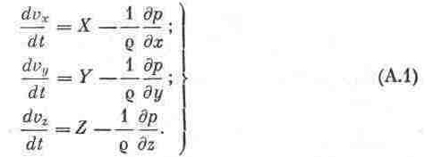
These equations were developed in 1755 by Leonhard Euler and bear his name. The terms represent the corresponding accelerations, the meaning of each equation being that the total acceleration of a particle along a coordinate axis is the sum of the acceleration due to body forces and the acceleration due to pressure forces.

Euler's equation is valid in this form for both incompressible and compressible fluids, as well as when gravity is the only acting body force and for relative motion of a fluid. In the latter case the quantities X, Y and Z must include the components of the acceleration in the transport or rotational motion.

For motionless fluid,

and Euler's equations take the form

These are the differential equations for fluid equilibrium.