

Explain the shapes of Marginal cost and Average total cost (why mc rising & atc u-shaped) and then explain the relationship between them (mc & atc). Prove your answer on the graph as well.
Marginal cost rises with the quantity of output produced. This reflects the property of diminishing marginal product. When producing a small quantity, producer has few workers, and much of his equipment is not being used. Because he can easily put these idle resources to use, the marginal product of an extra worker is large, and the marginal cost of an extra product is small. By contrast, when producing a large quantity of product, his stand is crowded with workers, and most of his equipment is fully utilized. Producing more products by adding workers, leads new workers have to work in crowded conditions and may have to wait to use the equipment. Therefore, when the quantity of product being produced is already high, the marginal product of an extra worker is low, and the marginal cost of an extra product is large.
Average-total-cost curve is U-shaped. Average total cost is the sum of average fixed cost and average variable cost. Average fixed cost always declines as output rises because the fixed cost is getting spread over a larger
number of units. Average variable cost typically rises as output increases because of diminishing marginal product. Average total cost reflects the shapes of both average fixed cost and average variable cost. At very low levels of output average total cost is high because the fixed cost is spread over only a few units. Average total cost then declines as output increases. The bottom of the U-shape occurs at the quantity that minimizes average total cost. This quantity is sometimes called the efficient scale of the firm.
Whenever marginal cost is less than average total cost, average total cost is falling. Whenever marginal cost is greater than average total cost, average total cost is rising. The marginal-cost curve crosses the average-total-cost curve at the efficient scale.
If a firm operating in the area of Constant returns to scale, what will happen to average total costs in the short-run if the firm expands production? What will happen to average total costs in the long run? Show on the graph your answers.
Because many decisions are fixed in the short run but variable in the long run, a firm’s long-run cost curves differ from its short-run cost curves. The long-run average-total-cost curve is a much flatter U-shape than the short-run average-total cost curve. All the short-run curves lie on or above the long-run curve. These properties arise because of the greater flexibility firms have in the long run. In essence, in the long run, the firm gets to choose which short-run curve it wants to use. But in the short run, it has to use whatever short-run curve it chose in the past.
While a firm operating in the area of Constant returns to scale, if it expands production, average total cost in the short - run will increase with the price, while in Long- run it will not change, except quantity.
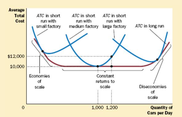
When a small firm expands the scale of its operation, why does it usually first experience increasing returns to scale (Economies of scale)? When the same firm grows to be extremely large, why might a further expansion of the scale of operation generate decreasing returns to scale (Diseconomies of scale). Also demonstrate your answer on the graph with your own example.
The shape of the long-run average-total-cost curve conveys important information about the technology for producing a good. When long-run average total cost declines as output increases, there are said to be economies of scale. When long-run average total cost rises as output increases, there are said to be diseconomies of scale. When long-run average total cost does not vary with the level of output, there are said to be constant returns to scale. Economies of scale often arise because higher production levels allow specialization among workers, which permits each worker to become better at his or her assigned tasks.
Diseconomies of scale can arise because of coordination problems that are inherent in any large organization.
Chapter 15