

Aggregate Demand and Aggregate Supply. Model ad-as. Совокупный спрос и совокупное предложение.
A ggregate
demand (AD)
is the total demand for final goods and services in the economy (Y)
at a given time, price level and inventory levels. Elements:
C consumption spending, I investment spending, G government
transfers, X export, IM import, as the GDP equation (GDP=C+I+G+X-IM)
can be considered as the quantity of domestically produced final
goods & services demanded during the year in case of constant
prices. The
aggregate demand curve
shows the relationship between the aggregate price level and the
quantity of aggregate output demanded.
ggregate
demand (AD)
is the total demand for final goods and services in the economy (Y)
at a given time, price level and inventory levels. Elements:
C consumption spending, I investment spending, G government
transfers, X export, IM import, as the GDP equation (GDP=C+I+G+X-IM)
can be considered as the quantity of domestically produced final
goods & services demanded during the year in case of constant
prices. The
aggregate demand curve
shows the relationship between the aggregate price level and the
quantity of aggregate output demanded.
It is downward-sloping for two reasons. Wealth effect of a change in the aggregate price level—a higher aggregate price level reduces the purchasing power of households and reduces consumer spending. Interest rate effect of a change in aggregate the price level—a higher aggregate price level reduces the purchasing power of households, leading to a rise in interest rates and a fall in investment spending. Shifts: Increases (rightward) when consumers and firms become more optimistic (change in expectations), the real value of household assets rises (change in wealth), the (change in) existing stock of physical capital is relatively small, the government increases spending or cuts taxes (change in fiscal policy), and the central bank increases the quantity of money (change in monetary policy) and vice versa (leftward).
A
 ggregate
supply
is the total amount of goods and services that firms are willing to
sell at a given price level and time. The aggregate
supply curve
shows the relationship between the aggregate price level and the
quantity of aggregate output in the economy. The short-run
aggregate supply curve
is upward-sloping because nominal wages are sticky (slow to fall even
in the face of high unemployment and slow to rise even in the face of
labor shortages) in the short run: a higher aggregate price level
leads to higher profits and increased aggregate output in the short
run. Shifts:
Increases when commodity
prices
fall, nominal
wages
fall, workers become more productive
and vice versa.
ggregate
supply
is the total amount of goods and services that firms are willing to
sell at a given price level and time. The aggregate
supply curve
shows the relationship between the aggregate price level and the
quantity of aggregate output in the economy. The short-run
aggregate supply curve
is upward-sloping because nominal wages are sticky (slow to fall even
in the face of high unemployment and slow to rise even in the face of
labor shortages) in the short run: a higher aggregate price level
leads to higher profits and increased aggregate output in the short
run. Shifts:
Increases when commodity
prices
fall, nominal
wages
fall, workers become more productive
and vice versa.
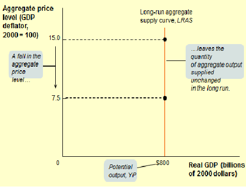
T he
long-run
aggregate supply curve shows
the relationship between the aggregate price level and the quantity
of aggregate output supplied that would exist if all prices,
including nominal wages, were fully flexible.
he
long-run
aggregate supply curve shows
the relationship between the aggregate price level and the quantity
of aggregate output supplied that would exist if all prices,
including nominal wages, were fully flexible.
T![]() he
AS-AD model
uses the aggregate supply curve and the aggregate demand curve
together to analyze economic fluctuations. There is a recessionary
gap
when aggregate output is below potential output, inflationary
when above. The economy is self-correcting when shocks to aggregate
demand affect aggregate output in the short run, but not the long
run.
he
AS-AD model
uses the aggregate supply curve and the aggregate demand curve
together to analyze economic fluctuations. There is a recessionary
gap
when aggregate output is below potential output, inflationary
when above. The economy is self-correcting when shocks to aggregate
demand affect aggregate output in the short run, but not the long
run.
S tabilization
policy
is the use of government policy to reduce the severity of recessions
and rein in excessively strong expansions. Policy
dilemma in the face of supply shocks:
a policy that counteracts the fall in aggregate output by increasing
aggregate demand will lead to higher inflation, but a policy that
counteracts inflation by reducing aggregate demand will deepen the
output slump.
tabilization
policy
is the use of government policy to reduce the severity of recessions
and rein in excessively strong expansions. Policy
dilemma in the face of supply shocks:
a policy that counteracts the fall in aggregate output by increasing
aggregate demand will lead to higher inflation, but a policy that
counteracts inflation by reducing aggregate demand will deepen the
output slump.
The high cost — in terms of unemployment — of a recessionary gap and the future adverse consequences of an inflationary gap => Active stabilization policy, using fiscal or monetary policy to offset shocks.