

Models and methods of multiprojekts managment - Vladimir N. Burkov, Dmitri A. Novikov
.pdfKeywords: project management, resource allocation, network planning
Vladimir N. Burkov, Dmitri A. Novikov
MODELS AND METHODS OF MULTIPROJECTS’ MANAGEMENT
The paper deals with the problems of resource allocation between several independent projects. The problem is to minimise the time of all the projects implementation or the weighted sum of termination times. The described approach is based on the representation of a project as the separate operation. Then the problem of optimal resource allocation between the operations is solved. Given resource allocation for every project, one can solve the problem of allocation inside the multiproject. Allocation and aggregation methods are explored.
INTRODUCTION
The development of the society, economy, enterprise and the development of the certain man may be represented as the set of discrete processes with given terminal goals under the constraints on time and resources. It is convenient for a man to divide the process of his activity on local processes. Projects are processes of changes, i.e. nonrepeated processes, which require for their implementation special methods of management. For example, regular morning exercising is not a project as it is repeatable and does not require special organisational efforts. But learning new morning exercises may be considered as a project. Daily production on the enterprise is not the project too, but introduction of new technology is a project. Evidently, the difference is not obvious - construction of the building is a project, but there is no reason to consider the standard block lodges production with their installation on certain place as a project.
In the former Soviet Union project management was broadly used since the end of 60-th and was referred to as the network planning and management. The base of project management is the presentation of the project network
graphic, which reflects the dependence between different operations of the project. In 70-th the interest to the methods of network planning and management decreased, as the reasons of nonefficient management were deeper - they laid in the basis of the public-political and economic principles of state. Nowadays in Russia project management outlives a second birth. The Russian Association of Project Management (SOVNET) is the member of the International Project Management Association (INTERNET).
Multiprojects are an important class of projects. Multiproject is a project, which consists of several technologically independent projects, united by the shared resources (financial or material, etc.). This paper considers methods and mechanisms of multuprojects management. The described approach is based on the presentation of a project as the separate operation. Then the problem of optimal resource allocation between the operations is solved. Given resource allocation on every project, one can solve the problem of allocation for the multiproject (between the projects - operations of the multiproject). Several allocation and aggregation methods are explored below.
1.RESOURCE ALLOCATION
BETWEEN INDEPENDENT OPERATIONS
Consider the multiproject, which consists of n independent projects. Each project is aggregately described as the operation with two characteristics: the volume of the project - Wi and the dependence between the rate of project implementation wi(t) = fi(ui(t)) and the amount of resources ui(t) at time t. The volume, the velocity and the termination time Ti are interconnected trough the following equation:
Tòi |
fi [ui (t)]dt = Wi . |
(1) |
0 |
|
|
Let the total amount of resources for the multiproject is given and equals N(t). The problem is to allocate this resources between the operations so, that
2
the termination time T = max Ti be minimal. If for any t N(t)=N (even arrival of
i
resources) and fi(ui) are concave functions, the resource allocation problem has the solution, defined in [1, 2, 3]. It is well known that the optimal allocation is characterised by the following properties:
à) each operation is implemented under the fixed level of resources ui(t)=ui, i = 1÷n, t [0, T], i.e. with a fixed rate;
á) all the operations terminate simultaneously.
Thus, wi = Wi/T is a constant rate of i-th operation. Denote ϕi(wi) - the function, inversed to function fi(ui), then ui = ϕi(Wi/T) is the amount of resources to terminate i-th operation at time T. Minimal value of T is defined by the following equation
|
n |
æW ö |
(2) |
|||||
|
åϕ |
ç |
|
i |
÷ |
|
|
|
|
|
|
|
|
|
|||
|
i=1 |
i è |
|
T ø = N . |
|
|
|
|
|
|
|
~ |
~ |
|
|
||
|
|
|
|
|
||||
|
Let N(t) be piece wise constant function: N(t) = Nk, t [ Tk−1 |
, Tk ), k = 1, p, |
||||||
~ |
= 0. Fix some k and consider the problem of multiproject’s implementation |
|||||||
T0 |
||||||||
|
~ |
|
- the volume of i-th operation, implemented |
|||||
at the time, less than Tk . Denote xiq |
||||||||
in the q-th interval. Obviously |
|
|
|
|
|
|
|
|
|
|
k |
|
|
|
|
|
|
|
|
åxiq = Wi . |
(3) |
|||||
q=1
As in the interval [Tq-1, Tq) the resources arrive evenly, the values {xiq} in the optimal solution satisfy the following constraint:
n |
æ xiq ö |
|
|
~ ~ |
||
|
|
|
||||
|
ç |
|
÷ |
= Nq , q = 1, k -1, Tq = Tq - Tq−1 |
||
|
|
|||||
åji ç |
T ÷ |
|||||
i=1 |
è |
q ø |
|
|
|
|
and for the last interval the following condition holds:
n |
æ xik ö |
~ ~ |
|
||
|
|
||||
åji ç |
|
÷ |
= Nk , T = T - Tk 1 |
, |
|
|
|||||
i=1 |
è |
T ø |
− |
|
|
|
|
|
|
|
|
where T is the time of all the operations termination.
3

Denote hq - the vector with components hiq = ji’(wiq), i = 1, n . The vector h is «time-invariant» (its direction does not alter with the change of time interval, while its length changes):
hq = γ q h1 , q = 2, k , h1 = {hi }, γ 1 = 1.
This characteristic of the optimal solution allows to reduce the resource allocation problem to the solution of the non-linear equations system with (n + k) variables {hi}, i = 1, n , {gq}, and T:
n |
|
||||
åji [xi (g q × hi )]= Nq , q = |
|
|
|
|
|
1, k |
(4) |
||||
i=1 |
|
||||
k−1 |
|
||||
åxi (g q × hi ) × Tq + xi (g k × hi ) × T = Wi , i = |
|
. |
(5) |
||
1, n |
|||||
q=1
Let fi(ui) are concave functions, then, given the total amount of resources (financing) for the interval [0, T], maximum of the implemented operations volume is reached under even (homogenous) resources arrivement. The proved fact allows to optimise the schedule of resources arrivement. Such a tuning may be achieved by the shift of financing on later periods.
Hitherto we considered the problem of multiproject time minimisation. However, the other problem is not of the less important. The matter is that after the termination of any project one should receive some income. The delay in the termination leads to the decrease of income. Assume that i-th project returns after its termination the income ci per time unit. Then the possible decrease of the income (lost income) is citi, while the total decrease equals
n |
|
C = åci ti . |
(6) |
i=1
Thus the following problem arises: to allocate resources between the projects to minimise (6).
4
2. THE GENERAL CASE
Above we have considered the problem of resource allocation under the assumption that the rate of project implementation is a concave function of the
resources amount. Now we turn to the general case. |
|
Let fi(ui) be some limited, continuos on the right functions, |
such that |
fi(0)=0. Define the set Y of pairs (u, w) in the following way: |
|
Yi = {(ui , wi ) > 0: wi ≤ fi (ui )}. |
(7) |
Note, that if fi(ui) is a concave function, then Yi is a convex set. Generally Yi is
not a convex set. The convex shell of this set is the convex set ~ , such that any
Yi
point may be represented as the convex linear combination of the points from
the set Yi. The border ~i ( i ) of this set is, obviously, a concave function.
u
f
Consider the resource allocation problem for the multiproject with the following
rates of projects implementation { ~i ( i )}. Suppose, that we have some optimal
f
u
allocation {ui0} and operations termination times { ti }.
Theorem 1. There exists feasible resource allocation with the same operations termination times ti.
3.AGGREGATION METHODS
FOR A COMPLEX OF OPERATIONS
Consider the methods of the complex of operations description in the form
of some unique operation. One should determine the volume of the aggregated operation Wý, which is referred to as the equivalent volume of the complex, and the dependence between the rate of the aggregated operation implementation and the amount of resources, allocated for the complex:
Wý(t) = Fý(N(t)) (8) Definition. Aggregation is identified as ideal if for any function N(t) there exists optimal resource allocation {ui(t)} between the operations of the complex,
such that
5

n
åui (t) £ N(t) ,
i=1
meanwhile minimal termination time of the complex satisfies the following condition:
Tmin |
|
ò Fэ (N(t))dt = Wэ . |
|
0 |
|
The classical example of the ideal aggregation is the following : |
|
fi (ui ) = uαi , a £ 1, i = 1, n. |
(9) |
Really, for this case it was proved [3], that there exists equivalent volume Wý of the complex and the function
Fý(N) = Nα,
such that for any resources level N(t) the following condition holds
Tmin
ò F[N(t)]dt = Wэ .
0
Herewith, there exists optimal allocation {ui0(t)}, such that
n
åu0i (t) = N(t),
i=1
and complex’s termination time equals Tmin.
Let for any t N(t) = N, then the allocation {ui0(t)} possesses the following interesting characteristics:
1. Each operation is implemented without any breaks with the constant amount of resources, i.e.
u0i (t) = ui , t Î[tHi , t0i ],
where tiH, ti0 are moments of the i-th operation beginning and termination. 2. The resources {ui} form the flow on the network graph.
Let us describe the algorithm of the equivalent volume of the complex determination. First one should define the dependence between costs Sij = uij×tij and operation’s time:
6

|
|
|
|
æ wij ö 1α |
|
wij1α |
|||
S |
ij |
= t |
ij |
× ç |
|
÷ |
= |
|
|
|
|
1ij−α α |
|||||||
|
|
è |
tij ø |
|
t |
||||
Consider the problem of optimising the complex by cost: to determine operations times to implement the complex in time Ò with minimal costs
S = åSij (tij ). |
(10) |
(i,j) |
|
å |
|
dSij (tij ) |
= å |
dS |
ki |
(t |
ki |
) |
. |
(11) |
||
|
dtij |
dtki |
|
|
|
|||||||
j |
k |
|
|
|
|
|||||||
|
|
|
|
|
|
|
|
|
|
|
|
|
Wý = TNα = Sαmin×T1-α
Let us describe another method of the equivalent complex’s volume estimation. This method is based on the following theorem:
7

Theorem 2. Equivalent volume of the complex is a convex homogenous function of operations volumes W .
The theorem allows to obtain overestimates of the equivalent volume of the complex, due to the presentation of the complex in the form of the convex linear combination of other complexes with known equivalent volumes.
Example. Consider the complex of operations, presented of fig. 1. The precise value of complex’s equivalent volume equals Wý = 3
 41 ≈ 19,2.
Consider two complexes of operations, presented on fig. 2 à, b. It easy to see that the average of this complexes volumes gives the first complex. For the second complex we obtain
Wэ1 = 
 212 + 132 ≈ 24,7 , and for the complex from fig. 2.b:
Wэ2 = 
 112 + 82 + 5 ≈ 18,6. Thus for the original complex:
Wэ ≤ 21 (Wэ1 + Wэ2 ) = 21,6.
The deviation from the precise estimate is 2,4 or approximately 12,5%. Accuracy of the estimate may be improved by the selection of different
values W1, W2 and α, such that
W = αW1 + (1 - α)W2.
8
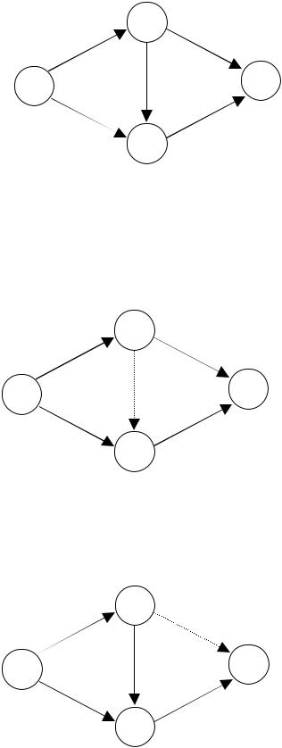
1
0 |
3 |
|
2
Fig. 1.
|
1 |
(5) |
(16) |
0 |
3 |
|
|
(8) |
(10) |
|
2 |
Fig. 2.à
1
|
(5) |
|
0 |
(6) |
3 |
|
|
|
|
(8) |
(5) |
|
2 |
|
Fig. 2.b
9
For example, if a » 1, then:
Wý1»18, Wý2 »3/(1-a), Wý £ 18 + 3 = 21, i.e. the deviation is approximately 9%.
4. THE LINEAR CASE
Consider the linear dependence between the rates of operations and the amount of resources:
ìui , |
ui ≤ ai |
. |
fi (ui ) = í |
ui ³ ai |
|
îai , |
|
Denote ti = wi/ui - the minimal time of i-th operation. Let us construct the integral graphic of resource utilisation on the complex of operations under the assumption that all the operations are initialised at the latest time moments. Graphic of resources utilisation is an aggregated description of the project. Really, given the aggregated descriptions of all the projects (right-shifted graphics of the projects), we are able to solve the problem of the optimal resource allocation for the multiproject both for the criteria of time minimisation and for the lost income minimisation.
Time minimisation problem for the multiproject is solved rather simple. Let Si(t,T) be the integral graphic of i-th project resources utilisation under the
n
condition of its termination at time moment T, S(t,T) = åSi (t,T) - the integral
i=1
graphic of multiproject resources utilisation, M(t) - the integral graphic of total amount of resources (fig.. 3).
10