Management of active systems stability or efficiency - Dmitriy A.Novikov

Keywords: active systems control, model’s adequacy, solution stability, incentive problem.

Abstract

The analysis of the solutions stability, as well as the analysis of models adequacy, is performed on the basis of the unified approach, which exploits the concept of the generalised solution of the active systems (organisational or socio-economic systems) control problem.

1. The model of the active system

Consider the problem of management in the active system (AS), which consists of the principal and the agent [1]. The state of the AS is described by the action of the agent - the variable y Î A, which belongs to the set of the feasible actions A. The action of the agent depends on the control variable u Î U, u = uˆ( y) : y = F(u). The function F(u, y), defined on

the set U ´ A, reflects the efficiency of the AS functioning. Thus K(u) = Φ(u, F(u)) is the efficiency of the control

u Î U.

Principal's management problem is to choose the control u*, which maximises the efficiency, given the response F(×) of

the AS: K(u) → max . u U

Game-theoretical problem is formulated as following. Agent's goal function f(y, u) reflects his preferences over the set A´U and depends on his own strategy y Î A and on the strategy u Î U of the principal. Define P(u, f) - the game solution set (the set of the implementable actions) as the set of the equilibriums under the given control u Î U. In the singleagent AS this set coincides with the set of the maximums of his goal function, in the multi-agent AS it is the set of Nash or Bayes equilibriums [1].

The set of the implementable actions corresponds to the principal's assumptions about the behaviour of the agent. Moreover, the principal (whose interests are identified with the interests of the whole AS) must specify his beliefs towards certain strategies of the agent, chosen from the set P(u, f). Two extreme approaches are mostly common used - the principle of the maximal guaranteed result (MGR - when the principal expects the worst from his point of view choice of the agent) and the hypotheses of benevolence (HB - when the principal expects the best from his point of view choice of

the agent), which is assumed to be valid through the consequent exposition.

The control (as the formal description is considered below, the term "control" is used instead the term "management") problem under the HB is formulated as

Two important cases of the control problem are the incentive problem and the planning problem. In the incentive problem the control variable uˆ (×) corresponds to the mapping from the set of the feasible actions onto the set of the feasible rewards [4-6], in the planning problem it corresponds to the mapping from the set of feasible messages, send by the agents onto the set of the feasible collective decisions [1].

When formulating the game-theoretical control problem, we implied that the model of the AS coincides with the real AS. Let's consider the possible differences between the AS and its model.

Introduce the following assumption: the model of the AS completely complies with the real AS in all parameters, except the goal functions of the principal and the agent and the sets of their feasible strategies.

Imagine the following situation. Let the control problem is solved for some model of the deterministic AS (see the models under interval, stochastic and fuzzy uncertainty in [3- 6]) under the assumption that all of the model parameters exactly coincide with the parameters of the real AS. What may happen if the parameters of the model "slightly" differ from parameters of the real AS?

Thus it may turn out to be that the problem has been solved for "another" AS and one can not a'priori deny this possibility. So it is necessary to get the answers on the following questions:

-is the optimal solution sensitive to the disturbances of the model description, i.e. will the "small" disturbances lead to the adequately "small" changes in the solution (conditionally we'll refer to this problem as the problem of solution's stability);

-will the optimal (in the framework of the model) solution remains optimal in the real AS (conditionally we'll refer to this problem as the problem of model's adequacy).

2.The stability of the active systems control problem solutions

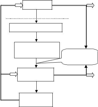
Consider the process of mathematical modelling (see Figure 1). The first step is the choice of the "language", which is used in the description of the model, i.e. the choice of the mathematical apparatus, which will be used (horizontal line in Figure 1 is the virtual border between the reality and the models). Usually this step is characterised by a high level of abstraction – a class of models is much broader than the modelled system. A possible mistake, which may be made by the operation researcher is the choice of the inadequate language of description.

Figure 1. Steps of AS mathematical modelling

Observed behavior

The next step is the construction of the set of particular models, which require certain assumptions about the general properties of model components. Mistakes, immanent to this step, may be caused by the improper beliefs about the properties of the modelled system components and their interaction.

Given model's structure, the operation researcher has to choose certain values of model's parameters (including numerical values). Thus some model is obtained and just this model is considered as the analogue of the real (modelled) system. The source of the "measurement errors", which arise in this step, is obvious and well explored (at least for technical systems) in the identification theory.

When the optimal control problem is solved for certain model, "computational errors" arise.

The problem of the solutions stability, studied in the operation research [2], is connected with the "distortions", caused by the "measurement errors" and "computational errors", and is solved by the analysis of the optimal solution dependence from the parameters of the model. If this dependence is continuous, then small errors lead to the small deviations of the solutions. Then, solving the control problem

on the basis of ill-defined data, one may be sure to find the approximate solution. If the dependence of the optimal solution on the parameters of the model is not continuous, or the solution is not defined in some vicinity of the exact solution, one have to apply the regularisation methods [2, 3].

What may be treated as the adequacy of the model? The solution, which is optimal in the model, being applied to the real system, is expected to lead to the optimal behaviour of the AS (see Figure 1). But, as the model may differ from the real AS, the application of this solution to the real AS generally leads to some (observed) behaviour of this AS. Obviously, the expected and the observed behaviour may differ greatly. Consequently, it is necessary to explore the adequacy of the model, i.e. to explore the stability of the real system behaviour (but not the stability of the model behaviour) towards the mistakes of modelling.

Consider the formal definitions.

Let M be the set of AS models which includes the real AS

~ ~

m, as well as its model m (the index « » corresponds to the variables of the model). The model (and the real AS) may be

feasible sets of the principal and the agent, so the criterion of

the control efficiency ( ~ ) depends on the model

K u, m

(remember that above the model of the AS was reflected by the "response" mapping F(×)).

Suppose (until it will not be specially noted below) that the model may differ from the original only in the preferences

To describe models closeness, introduce the pseudometric m - numerical function, defined on M ´ M, such that:

"m1,m2m3ÎM m(m1,m1)=0, m(m1,m2)+m(m2,m3)³m(m1,m3). Introduce the criterion principle of optimality, induced by

the efficiency criterion K(u, m), u Î U, m Î M. As optimal (accurately, e-optimal, e³0) strategies form the following set:

the corresponding principle of optimality is referred to as the criterion principle of optimality [2].

The problem of the optimal (i.e. "classically" optimal, e = 0) control consists of the looking up the feasible control, which maximises the efficiency for given AS or its model:

Thus the set R0(m) of solutions corresponds to the "classical" principle of optimality K(m).

Let U is a metric space with the metric n. This metric generates the Hausdorf's metric Hn(B1, B2) [2], which defines the "distance" between the subsets B1 and B2 of the set U.

Lyapunov's definition and qualitatively means that the small distortions of the model lead to the small changes in the optimal solutions.

Criterion optimality principle Rε(m) is considered to be

~ Î

stable on the model m M if the function K(m) (see (2)) is

~

continuous on the model m .

The domain of the absolute stability may be defined as:

B(e, u) = {m Î M | u Î Rε(m)}.

Qualitatively, the absolute stability of the certain solution (which is e-optimal in the model m~ ) in some domain means that it is e-optimal in any other real AS (and its model) from this domain. Obviously " u Î U, " e1 ³ e2 ³ 0 B(0, u) Í B(e2, u) Í B(e1, u), i.e. with the increase of e the domain of the absolute stability of some certain solution does not decrease.

3. Adequacy of the active systems models

Fix some model m~ Î M and the optimality principle Rε. Intuitively, if e = 0, then the adequacy corresponds (contrary

to the stability, when the continuity of sup K(t, m) on the t M

i.e. to that real AS, where at least one of the solutions, which are optimal in the model, is optimal too. In other words, the model m~ with the optimality principle Rε is e-adequate to the set of real AS Mε( m~ ) if $ u Î U: m Î B(e, u), m~ Î B(e, u) (or Mε( m~ ) Ç Mε(m) ¹ Æ). Hence the adequacy of the model is defined through the absolute stability of the corresponding optimal solutions.

Note, that the definition (5) is symmetric with respect to

{u Î U; B(e, u)} was named the generalised solution of the

problem for the model m~ Î M.

The above definition of the generalised solution is broad enough as it exploits the set of all e-optimal (in the model and in the real AS) solutions. Hence for any solution u Î U, apart from its efficiency (the efficiency of control, whose "feasible" deviation from the maximal value depends on the parameter e), there exists another characteristic - the set B(e, u) of AS, in which it is e-optimal, i.e. absolutely stable.

of those AS, for which any solution, which is e-optimal in the model, is also e-optimal.

Thus the possibility of the optimal solutions comparison arises. It is natural to consider, that for two solutions, satisfying the optimality principle, the solution that has the "larger" domain of absolute stability is "better". Introduce the

following relation "Ð" (which is generally incomplete) on the

the relation "Ð".

Thus for the fixed model and the principle of optimality one may point out the set of real AS (the set of models), in which there exists the solution, which surely satisfies the optimality principle. This set is undoubtedly not empty, as it includes the model itself.

If there exists the solution, which is e-optimal in the real AS as well as in its model, then the model may be considered to be adequate (e-adequate). Thus the criterion of model's ε- adequacy is the efficiency of the real AS control.

Moreover, the process of the model's analysis may be considered complete iff for any solution, satisfying the optimality principle, the sets of stability are indicated.

The knowledge of the set B(e, u), u Î Rε( m~ ), allows to estimate possible losses from the practical application of the results of modelling and (if it is necessary) to revise the model or the optimality principle.

The modification of the optimality principle looks very perspective, even under the fixed parameters of the model. For example, reducing the requirements to the efficiency, one can increase the domain of the solution stability and, consequently, increase the set of real AS, in which the solutions, satisfying the relaxed principle of optimality, will be guaranteed e-optimal (generally, the principle of e- optimality regularise the "classical" principle of optimality [2, 3, 7]).

Qualitative reasoning, presented above witness that there exists the dualism between the efficiency of the control and its stability. Trading the efficiency, one can increase the set of real AS, in which the results of modelling may be applied. This effect reveals itself brightly in the analysis of the stability domains. The value of e, appearing in the definition of the principle of optimality, characterises the losses in the efficiency, which we are ready to admit.

The dualism between the efficiency and the stability may be formally stated as following (see also the theorem below): the set of AS, which are adequate to the fixed model, does not decrease with the increase of e (and vice versa), moreover - the set of absolute stability of the fixed optimal (in the model) solution does not decrease with the increase of e [3, 7].

This fact (relaxing the requirements to the efficiency of some solution, one can increase the domain of its absolute stability and, consequently, increase the domain of adequacy) demonstrates that to solve the problems of stability and adequacy it is sufficient to point out concrete dependency between the value of e and the set of AS.

Constructive application of the generalised solutions to the incentive problem is described in the following section.

4.Generalised solutions of the incentive problem

Consider the following deterministic incentive problem: interests of the principal and the agent are reflected by their goal functions: F(y) = H(y), f(y) = h(y) - uˆ (y), H(y) -

principal's income, uˆ (y) Î U - incentive (or penalty) function, h(y) - agent's income. Principal's strategy is the choice of the incentive function uˆ (×), agent's strategy is the choice of the action y Î A. The set of the implementable actions is:

P(u) = Arg max {h(y) - uˆ (y)}. y A

Introduce the following assumptions:

А1. A = [0; A+] Í Â1, A+ < +¥;

А2. h(y) - single-peaked function [3] with the peak r Î A;

А3. U = { uˆ | " y Î A 0 £ uˆ (y) £ C};

А4. H(y) - single-peaked function with the peak r' ³ r.

Denote y+ = max {y Î A | h(y) ³ h(r) - C},

g³ 0;

-agent's income function h(y) may, staying single-peaked,

differs from the model in the given range. This numbers influence on the guaranteed efficiency of control e(g, d, b, x), correctly defined below (see (8)-(10) and the theorem).

Generalised solution of the deterministic incentive problem is given by the following statement (see analogues in [3, 7]).

References

1.Burkov V.N., Novikov D.A., Active systems theory. Moscow: Sinteg, 1999. (in Russian).

2.Molodtsov D.A., Stability of the optimality principles. Moscow: Science, 1987. (in Russian).

3.Novikov D.A., Generalised solutions of the incentive problems. Moscow: Institute of Control Sciences, 1998. (in Russian).

4.Novikov D.A., Incentives in organisations: uncertainty and efficiency, Proceedings of 6-th IFAC Symposium on Automated Systems Based on Human Skills, Kranska Gora, 274-277, (1997).

5.Novikov D.A., Incentives in socio-economic systems. Moscow: Institute of Control Sciences, 1998. (in Russian).

6.Novikov D.A., Project management and incentive problems, Proceedings of XII International Conference on Systems Science, Wroclaw, 2, 387-391, (1995).

7.Novikov D.A., Stability of the solutions and adequacy of the deterministic incentive models in active systems,

Automation and Remote Control, 7, 115 -122, (1999).