


C H A P T E R 8
Competition
Introduction
Interspecific competition has been the subject of almost as much acrimonious debate in ecology as has density dependence (Connor & Simberloff, 1986; Diamond, 1986; Connell, 1983; Roughgarden, 1983; Simberloff, 1983). The basic principle that two coexisting species will have a negative impact on each other, if they share a limiting resource, is not in dispute. However, inferring the strength, or even the existence, of competitive interactions using data from undisturbed field populations is difficult, and experiments designed to measure its impact are often trenchantly criticized (Underwood, 1986).
The simplest model of interspecific competition is the Lotka–Volterra model. It models two species N1 and N2, each independently following logistic growth with intrinsic growth rates r1 and r2 and carrying capacities K1 and K2. The presence of each species also has an impact on the carrying capacity of the other via competition coefficients α12 and α21. The equations can be expressed in various forms, including:
dN |
|
|
|
|
|
|
|
N |
+ α |
12 |
N |
2 |
|
|
|
|
|
|
|
|
|||||
1 |
|
= r N |
1 |
− |
|
1 |
|
|
≡ f (N |
,N |
), |
(8.1) |
|||||||||||||
|
|
|
|
K |
|
|
|
||||||||||||||||||
dt |
|
|
1 |
1 |
|
|
|
|
|
|
|
|
|
|
|
1 |
1 |
|
2 |
|
|
|
|||
|
|
|
|
|
|
|
|
|
|
|
1 |
|
|
|
|
|
|
|
|
|
|
|
|
||
dN |
2 |
|
|
|
|
|
|
|
N |
2 |
+ α |
|
N |
|
|
|
|
|
|
|
|
|
|||
|
|
= r N |
1 − |
|
|
|
|
|
21 1 |
|
≡ f |
(N |
,N |
|
). |
(8.2) |
|||||||||
dt |
|
|
|
|
|
K |
|
|
|
||||||||||||||||
|
|
2 |
2 |
|
|
|
|
|
2 |
|
|
|
|
2 |
1 |
|
2 |
|
|
||||||
|
|
|
|
|
|
|
|
|
|
|
|
|
|
|
|
|
|
|
|
|
|
|
|
||
From these, it can be seen that the competition coefficient α12 measures the effect of species 2 on the growth rate of species 1 relative to the impact of species 1 on its own growth rate. Whereas one individual of species 1 decreases the growth rate of its own species by a factor 1/K1, each individual of species 2 decreases the growth rate of species 1 by an amount α12/K1. This is a very general and abstract representation of interspecific competition, which can be extended to any number of species in a fairly obvious fashion.
It is easy to become confused about the meaning of subscripted parameters. The first subscript is the target of the competition, and the second the agent. Thus αij measures the effect of species j on species i. The distinction between αij and αji is important, as empirical evidence suggests strongly that competition is often very asymmetric (Lawton & Hassell, 1981; Connell, 1983).
216

C O M P E T I T I O N 217
The main use of this general model is to answer general questions, and most basic ecology textbooks provide a discussion of the competitive exclusion principle and conditions for coexistence of competitors based on this simple model (e.g. Krebs, 1985; Begon et al., 1990). Box 8.1 reviews the use of phaseplane analysis to study the behaviour of the model.
Box 8.1 Phase-plane analysis of the Lotka–Volterra competition equations
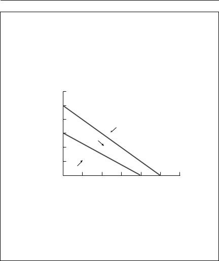
Phase-plane analysis is a powerful graphical method for exploring the qualitative behaviour of two-species differential equation models. A phase plane is simply a graph with the population size of one species on the horizontal axis, and the population size of the other on the vertical axis. Any point on the graph then represents a pair of species abundances. An arrow at that point can be used to show the trajectory of the system, which is the direction in which the model predicts the densities will change. Lines along which the rate of change of one of the species is constant can also be drawn. These are called isoclines. The most useful isoclines are the zero net growth isoclines (sometimes simply called zero isoclines). The zero net growth isocline of species 1 is the line along which the growth rate of species 1 is zero. Where the zero isoclines for both species cross, there is an equilibrium, a point where the system will remain, if it is already there. Trajectories drawn around the isoclines can be used to investigate the stability of the equilibrium. The zero isoclines for N1 and N2 can be found by setting dN1/dt = 0 and dN2/dt = 0 and then solving each equation to give N2 in terms of N1.
For example, in the simple Lotka–Volterra eqns (8.1) and (8.2), the zero isocline for N1 is the solution of
1 − |
N1 + α12N2 |
= 0 N2 = |
K1 |
− |
N1 |
, |
|
|
|
||||
|
K1 |
α12 |
α12 |
|||
and the zero isocline for N2 is the solution of
1 − N2 + α21N1 = 0 N2 = K2 − α21N1.
K2
Both of these zero isoclines are straight lines. The zero isocline for N1 divides the phase space into two regions. Close to the origin, N1 is increasing, but beyond the line, it decreases. Similarly, the N2 isocline divides the phase space into two regions. Simple vector addition (‘nose to tail’) can be used to predict the overall trajectory of the system at any point.
continued on p. 218
218 C H A P T E R 8
Box 8.1 contd
There are four qualitatively different outcomes from this pair of isoclines, as shown in the phase plots below. In each of these, the N1 isocline is shown with a solid line, and the N2 isocline is dashed.
K1 |
> K |
2 |
and |
K2 |
> K . |
(i) |
|
|
|||||
α12 |
|
α21 |
|
|||
|
|
|
1 |
|
||
|
K1lα12 |
|
2 |
K2 |
|
N |
|
|
|
K2 |
K2lα21 |
|
N1 |
|
In this case, there is an equilibrium with both species present, and the trajectories show that it is stable. The two species can coexist. Careful inspection of the conditions shows that one additional member of each species has a bigger effect on its own species’ growth rate than it does on the growth rate of the other species: intraspecific competition is stronger than interspecific competition.
K1 |
< K |
2 |
and |
K2 |
< K . |
(ii) |
|
|
|||||
α12 |
|
α21 |
|
|||
|
|
|
1 |
|
||
|
|
|
|
|
|
|
|
K2 |
|
2 |
K1lα12 |
|
N |
|
|
|
K2lα21 |
K1 |
|
N1 |
|
continued on p. 219
C O M P E T I T I O N 219
Box 8.1 contd
Now the zero isoclines still intersect, but the trajectories show that the equilibrium is unstable. One species will replace the other, but which one wins depends on the initial conditions. Interspecific competition is stronger than intraspecific competition.
K1 |
> K |
2 |
and |
K2 |
< K . |
(iii) |
|
|
|||||
α12 |
|
α21 |
|
|||
|
|
|
1 |
|
||
|
K1lα12 |
|
2 |
K2 |
|
N |
|
|
|
K2lα21 |
K1 |
|
N1 |
|
In this case, the isoclines do not intersect, and the N1 zero isocline is further from the origin than is the N2 zero isocline. Species 1 will always outcompete species 2.
K1 |
< K |
2 |
and |
K2 |
> K . |
(iv) |
|
|
|||||
α12 |
|
α21 |
|
|||
|
|
|
1 |
|
||
This is the reverse of (iii). Species 2 will always outcompete species 1.
Several authors have attempted to understand and model particular competitive interactions through parameterizing the model. Such approaches are most likely to be useful when modelling competition between microbes or protozoa, rather than large, long-lived organisms. More commonly, the model is used as a caricature of a competitive interaction. An attempt is made to estimate a competition coefficient, and this is used to infer something about competition between the two species, without the full model actually being used to predict the time-course of an interaction between the two species.
Defining interaction coefficients
There are at least four ways that interaction coefficients between species can be defined (Laska & Wootton, 1998). These are:

220 C H A P T E R 8
1 Per capita direct effects that one single individual of one species has on one member of another species. If eqns (8.1) and (8.2) were, in fact, an accurate description of a competitive interaction, then the per capita effect of species 2 on species 1 would be α12r1/K1. Frequently, this will be scaled relative to the density-dependent effect that the target species has on itself, yielding simply the coefficient α12.
2 Elements in a Jacobian matrix, evaluated at equilibrium. This approach was originally advocated by May (1974b). The Jacobian matrix is a matrix of first partial derivatives of the functions describing the interaction, with respect to each of the population variables in turn. For example, for the model described by eqns (8.1) and (8.2), the matrix would be:
∂f1(N1,N2) |
|||
|
∂N1 |
|
|
|
|||
|
∂f2(N1,N2) |
||
|
|
|
|
∂N1 |
|||
|
|||
∂f1(N1,N2) |
|
|||
|
∂N2 |
|
|
|
|
|
, |
(8.3) |
|
|
∂f2(N1,N2) |
|
||
|
|
|
|
|
|
∂N2 |
|
|
|
|
|
|
|
|
evaluated at the equilibrium point (N*, N*). With a little algebra, the effect of
1 2
species 2 on species 1 would therefore be:
∂f (N*,N*) |
= |
−α r (K − α |
12 |
K |
) |
|
||
1 1 2 |
|
12 1 1 |
2 |
|
, |
(8.4) |
||
∂N2 |
K1(1 − α12α21) |
|
||||||
|
|
|
|
|||||
provided that an equilibrium with both species present exists.
Equation (8.4) appears a little messy. However, if it is scaled relative to the equilibrium population density of the target species, which is
|
N* = |
K1 − K2α12 |
, |
(8.5) |
|||
|
|
||||||
1 |
|
1 − α21α12 |
|
||||
|
|
|
|
||||
it becomes simply |
|
||||||
|
∂f1 |
= |
−α12r1 |
. |
|
|
|
|
∂N2 |
|
|
||||
|
|
|
K1 |
|
|||
This definition is well suited to theoretical investigations, as it provides a single quantity to measure the interaction strength, even if the effect of one species on the other is nonlinear. It is rather difficult to use empirically, as it describes the effect on species 1 of an infinitesimally small change in species 2, and it requires that the system should be in equilibrium before manipulation.
3 The inverted negative Jacobian matrix. If the interaction in question is embedded in a multispecies community, the actual effect of reducing the density of species j on species i may be quite different from the direct effect. For example, suppose three species, A, B and C compete with each other. If B competes with A, then one would expect that reducing the density of B would

C O M P E T I T I O N 221
allow A to increase. But suppose that the effect of B on A is small, compared with the competitive effect that B has on C, and suppose further that C competes strongly with A. Then reducing B’s density would allow C to increase. C would then compete with A, producing an overall detrimental effect on A. The effect of reducing B would then be the opposite of the beneficial effect expected from the direct competitive interaction. The elements in the Jacobian matrix (expression (8.3) above), inverted and multiplied by −1, measure the overall (direct and indirect) effect of a constant small perturbation in any of the species in the community upon each of the others.
4 The removal matrix. An obvious way to investigate a competitive interaction experimentally is to remove the putative agent of the competition, and then record the change in abundance of the target. Laska and Wootton (1998) suggest measuring the strength of the interaction simply as the change in abundance of the target species when the competitor is removed. Paine (1992) suggests scaling the change relative to the abundance of the target in the community without the agent present, and then expressing the effect per individual agent. The interaction strength Iij, representing the effect on target species i of removing the agent species j, would then be:
Iij = Nij+ − Nij− (8.6)
Nij− Nj
where Nij− is the abundance of the target i after the agent j has been removed, Nij+ is the abundance of the target i with j present, and Nj is the abundance of the agent before removal. (Note that in Paine (1992), ‘controls’ are treatments from which the agent has been removed, and ‘treatments’ have the agent still present. This is rather confusing!) For the simple Lotka–Volterra model of eqns (8.1) and (8.2),
I12 = −α12 . (8.7)
K1
Provided two species only are interacting, and the effect of competition is linear, all four of the above definitions thus are equivalent, subject to minor considerations of scaling. All real competitive interactions, however, are embedded in larger food webs. Indirect interactions may have a substantial influence on measured competition coefficients. In several of the few cases that have been looked at systematically (see below), isoclines have also been found to be nonlinear.
Estimating competition coefficients from resource usage
The most intuitively obvious way to estimate competition coefficients without direct experimentation is to use the extent of overlap in resource use. This idea

222 C H A P T E R 8
was proposed by McArthur and Levins (1968). They suggested
|
∑p h pjh |
|
|
α j = |
h |
, |
(8.8) |
∑p2 |
|||
|
h |
|
|
h
where there are h potential resources, and pih is the relative resource utilization of resource h by species i. The relative resource utilization pih is the fraction of all its resources that species i obtains from resource h. If resource utilization patterns of the two species are identical, then αij will equal 1, and it will be less than 1 as the patterns of usage differ. There are substantial problems in both defining and estimating the pih terms, but even if this is accomplished, the problem remains that eqn (8.8) is an index of resource utilization overlap. To use an index of resource overlap as an index of competition, it would be necessary to make some adjustment for the total amount of resource use of individuals from each species. Furthermore, resource overlap is neither a necessary nor a sufficient condition for competition (Holt, 1987). If a particular resource is not limiting, overlap in usage will not result in competition. Interference competition may also occur without resource overlap. Schoener (1974b) has a detailed discussion of this approach and its variants, and a more recent discussion can be found in Krebs (1989). Whilst the indices thus calculated may be useful as measures of resource overlap, they cannot be considered as measures of competition coefficients that might have value in predicting the outcome of competitive interactions in the field.
Experimental approaches
If they can be carried out at appropriate temporal and spatial scales, there is no doubt that experimental manipulations of the density of potential competitors are a more satisfactory way to study competition than is observation. The most obvious way to investigate competition experimentally is to remove the putative agent of competition entirely from some replicated experimental units, leaving matched intact replicates as controls. Some time later, the population size or density of the putative target of competition is then compared between treatments and controls. This basic approach has been taken in a number of studies. Fairly recent examples include Paine (1992), Pfister (1995) and Fox and Luo (1996). Each of these authors considered this removal method to be a standard against which other approaches could be compared.
Provided only two species are interacting, provided the isoclines are linear, and provided the system can be assumed to have reached equilibrium after manipulation, the competition coefficient can be estimated from the observed data using eqn (8.6). Each of these provisos needs discussion. I have already briefly mentioned the problem of indirect interactions. Bender et al. (1984)

C O M P E T I T I O N 223
discuss it in detail. In general, there are two possible types of perturbation experiment. In ‘press’ experiments, the agent of competition is removed, or altered in abundance, and is maintained at this new level indefinitely. Once a new equilibrium is reached, the change in abundance of the target species or community is compared between treatment and control replicates. In ‘pulse’ experiments, a perturbation is applied at a single time, and the shortterm response of the entire community, including both agent and targets, is recorded as the system returns to equilibrium. A pulse experiment would ideally involve a small perturbation, rather than a complete removal of the agent.
Press experiments measure the total effect of removal of the agent species from the community, and therefore include indirect, as well as direct effects. If you want to estimate the coefficients αij themselves, this poses a problem. In an n-species community, each would need to be perturbed, the response of every other species would have to be measured, and the resulting matrix of total effects manipulated to extract the interaction coefficients (Bender et al., 1984). If you are interested in a particular pair of species, this is a difficulty more of theoretical than practical importance. The question is usually how one species affects another, in their particular community context, rather than one of resolving all the pathways of that interaction. In any event, Lotka– Volterra models subsume indirect interactions via species not included explicitly in the model into the interaction coefficients. If you want to describe all interactions in a community, then the problem of indirect interactions cannot be ignored, and is difficult to resolve with press experiments.
Pulse experiments record the short-term response of each species in a community to a single perturbation away from equilibrium. They are therefore attempting a direct measurement of the change in dNi/dt in response to the perturbation. In principle, they should be able to estimate the components of the interaction equations, providing estimates of the direct interaction coefficients αij themselves (Bender et al., 1984). In practice, there are major problems in applying the pulse approach to measuring competition in the field, and it has rarely been used (but see Seifert & Seifert 1976; 1979). Ideally, the perturbation should be infinitesimally small, so that the response of the system in the neighbourhood of equilibrium is determined. For practical purposes, however, the perturbation needs to be substantial, to produce a response big enough to be detected over random variation.
Bender et al. (1984) suggest the following procedure to estimate interaction coefficients between a pair of species i and j, which may be components of a wider interaction community. This procedure should be able to deal with temporal variation in the intrinsic growth rates and carrying capacities of the two species, provided such variation is the same across replicates.
1 Divide the available replicates into matched triples.

224 C H A P T E R 8
2 Perturb the putative agent species j in one of each triple, perturb the putative subject of competition i in another, and leave the final member as an undisturbed control.
3 A short time later, measure NCi and NCj, the population size of the target and agent species in the control community. At the same time, also measure NTij and NTjj, which are the population sizes of the target and agent species in the matched treatment community in which j has been perturbed. Also measure NTii and NTji in the matched treatment community in which i has been perturbed.
4 Simultaneously, also estimate the per capita rates of change of each popula-
tion in the control and treatment communities. Call these rC , rC, rT, rT, rT |
||||
and rT. |
|
i |
j ii ij ji |
|
|
|
|
||
|
jj |
|
|
|
5 Estimate the interaction coefficients using |
|
|||
α j = |
(r Tj |
− rC)(NC − N T) |
(8.9) |
|
|
|
. |
||
(r T |
|
|||
|
− rC)(NCj − N jjT) |
|
||
This equation relies on estimating per capita rates of change, as well as actual population sizes. To measure a competition coefficient between a pair of species, it is necessary to manipulate both species, not just the putative agent of competition. This is necessary because the competition coefficient αij is defined as the impact that species j has on species i relative to the impact that species i has upon itself. Whatever its theoretical advantages, this method will be difficult to apply in practice, particularly to vertebrate populations. Rates of population growth are not easy to estimate (see Chapter 5), and will also inevitably fluctuate more in response to environmental noise and sampling error than will estimates of population size themselves.
How long should be left between the perturbation and measurement of the response? This is not a simple question, nor is the answer. Obviously, if it is left too long, the impact of the perturbation may have disappeared entirely. It is also possible to measure the impact too soon. The method is intended deliberately to measure direct, and not indirect effects. However, the most common form of competition is resource competition. This is often a form of indirect interaction, as the limiting resource or resources are often one or more species of organism. Whether the pulse perturbation method will detect resource competition depends on the characteristic time scale on which the resource dynamics operate. There are three possible situations: resource dynamics that are much faster than the exploiters; resource and exploiter dynamics on comparable time scales; and resource dynamics on a much slower time scale than the exploiters. If the resource responds more rapidly than the exploiter populations, then a pulse experiment with the response recorded after the resource has settled to a new equilibrium will measure resource competition coefficients correctly. If the resource responds slowly, then resource

C O M P E T I T I O N 225
competition will not be detected at all. If time scales are comparable, then it is important to include the resource species in the perturbation experiment
– see Bender et al. (1984) for a more detailed discussion.
Mapping competition isoclines
A few recent studies have attempted to determine the shape of competitive isoclines experimentally. Mapping the zero net growth isocline for species 2, subject to competition by species 1, requires experimentally holding the species 1 population size constant at several levels, and then determining, at each of these levels, the population size of species 2 at which there is no net growth in the population of species 2. This will never be easy to do directly. In principle, it would be possible to use an elaboration of the ‘pulse’ approach advocated by Bender et al. (1984). Another way of approaching the problem is to see if the competition coefficient α12, which measures the effect of one individual of species 2 on one individual of species 1, is the same for all densities of each species. If it is, then the isocline is linear. If not, then α12 is the gradient of the isocline, and the form of the isocline itself can be obtained by integration with respect to N2, provided α12 is a function of N2 alone.
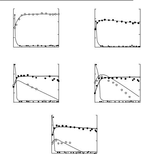
Abramsky et al. (1991; 1992; 1994) used an ingenious method to estimate the competition coefficients between two species of gerbil. They constructed replicated paired enclosures in the Negev Desert, Israel. Two gerbil species occupied the area: Gerbillus allenbyi (mean adult body mass about 26 g), and the larger G. pyramidum (mean adult body mass about 40 g). Their approach relies on the assumption that animals will distribute themselves between two different patches so that their average fitness is the same in each patch. This is the ‘ideal free distribution’ (Fretwell, 1972). If one further assumes that the per capita growth rate of a population is a measure of its average fitness, the animals should therefore distribute themselves so that the per capita growth rate is the same in each patch. If two patches differ only in that an agent of competition is present in differing densities, then the target of competition should distribute itself so that its density is higher in the patch where the competitor is less common than in the patch where the competitor is more common. The difference in the population density of the target species between the two patches, divided by the difference in density of the agent, is an estimate of the competition coefficient in that region of the state space.
To apply this method in practice, Abramsky and co-workers needed to devise a means of allowing one species of gerbil to move freely between adjacent enclosures, whilst constraining the other species to the enclosure into which they were placed. So that G. pyramidum could be prevented from moving between the paired enclosures, they used small gates through which only the smaller G. allenbyi could fit (Abramsky et al., 1992). Designing a means
226 C H A P T E R 8
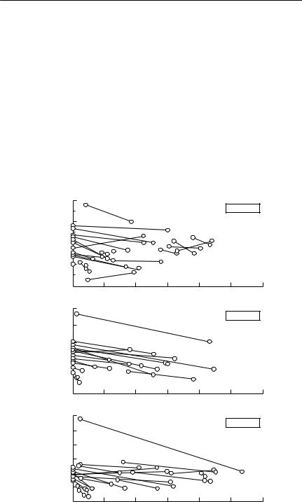
of allowing the larger G. pyramidum to move through gates, whilst constraining the smaller species was more difficult (Abramsky et al., 1994). They developed the ingenious device of weight-dependent latch mechanisms. The method requires that the quality of each enclosure must be identical, so that the animals should distribute themselves equally between the enclosures, if the competitor is not present. This is testable. It also requires that the animals should distribute themselves according to the ideal free distribution if a competitor is present in differing abundance between patches. This assumption cannot easily be tested, although Abramsky et al. (1991) use similar weight changes in animals in each pair of enclosures as evidence that fitness is similar in each pair.
The results Abramsky et al. obtained are shown in Fig. 8.1. If the animals do indeed distribute themselves so that their fitness is the same in adjacent enclosures, and stochasticity is neglected, then each of the lines shown in the
|
80 |
|
AGA |
60 |
|
of |
||
|
||
density |
40 |
|
Activity |
20 |
|
|
(ai) |
0 |
|
AGA |
100 |
80 |
|
of |
40 |
density |
|
|
60 |
Activity |
20 |
|
0
(aii)
AGA |
120 |
|
100 |
||
of |
80 |
|
density |
||
60 |
||
|
||
Activity |
40 |
|
20 |
||
|
0
(aiii)
Plots 3–4
10 |
20 |
30 |
40 |
50 |
60 |
Plots 5–6
10 |
20 |
30 |
40 |
50 |
60 |
Plots 7–8
10 |
20 |
30 |
40 |
50 |
60 |
|
Activity density of AGP |
|
|
||
AGAof |
100 |
|
|
|
|
|
|
80 |
|
|
|
|
|
|
|
|
|
|
|
|
|
|
|
density |
60 |
|
|
|
|
|
|
40 |
|
|
|
|
|
|
|
Activity |
|
|
|
|
|
|
|
20 |
|
|
|
|
|
|
|
|
|
|
|
|
|
|
|
|
0 |
10 |
20 |
30 |
40 |
50 |
60 |
(bi) |
|
|
|
|
|
|
|
|
100 |
|
|
|
|
|
|
Activity density of AGA
80
60
40
20 |
0 10 20 30 40 50 60
(bii)
100
Activity density of AGA
(biii)
80
60
40 
20 

0 |
10 |
20 |
30 |
40 |
50 |
60 |
|
|
Activity density of AGP |
|
|
||
Fig. 8.1 Competition coefficients for gerbils. The axes in the figure show the population density of Gerbillus allenbyi (AGA, vertical axis) and G. pyramidum (AGP, horizontal axis), as measured by an activity index based on track counts on sandplots. Abramsky et al. felt that this method of estimating density was less disruptive to normal behaviour patterns than a trapping-based index. In each graph, lines connect data from simultaneous censuses on adjacent plots, separated by a ‘semipermeable’ fence. The gradient of the lines connecting these pairs was used to estimate the competition coefficient in the region of the state space in which the line falls. Dashed lines identify the few cases where the gradients of the lines were positive. (a) G. pyramidum as the agent of competition (with densities fixed in each plot), and G. allenbyi as the target (free to move between members of a pair). The individual panels are for each pair of enclosures. (b) G. allenbyi as the agent of competition (with densities fixed in each plot), and G. pyramidum as the target (free to move between members of a pair). In this case, each panel represents a series of experiments carried out in different pairs, but in the same month. From Abramsky et al. (1992, 1994).
228 C H A P T E R 8
figure should be chords (straight lines) connecting points on an isocline for the species that is free to move. (Recall that an isocline for a species is a line in state space along which the species’ growth rate is constant.) All the lines will not be on the same isocline, however, and no line will necessarily be on the zero net growth isocline. However, each line will be an estimate of the gradient of an isocline in the region of state space sampled.
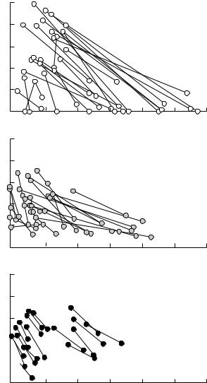
Abramsky et al. used regressions to predict the gradient of the isoclines as a function of the activity density of each species. They estimated activity density by the number of gerbil tracks left on sandplots. This index would estimate either actual density or total activity level with substantial error, potentially leading to substantial ‘measurement error bias’ (see Chapter 11). Their results are shown in Fig. 8.2. They then integrated the equations to obtain zero net growth isoclines for each species. To do this, it is necessary to specify a constant of integration, which determines where the isocline is located in state space. Zero net growth isoclines must pass through any equilibrium point, so forcing a zero isocline to pass through an observed equilibrium is an appropriate way to determine its constant of integration. Of course, this makes circular any attempt to ‘test’ the isoclines by seeing if they successfully predict the location of the observed equilibrium.
The zero isoclines presented by Abramsky et al. (1994) are shown in Fig. 8.3. Neither is linear, and the overall shape of each can be explained in terms of the habitat use and behaviour of the two species (see Abramsky et al., 1994, for details). The isoclines predict that the leftward equilibrium where both species coexist should be only locally stable: if G. pyramidum activity density increases beyond a breakpoint of about 45, G. pyramidum should be able to exclude G. allenbyi. There is some anecdotal evidence consistent with this prediction.
This method offers the possibility of experimentally estimating the shape of isoclines from field data. However, it relies totally on the assumption that the animals will distribute themselves in accordance with the ideal free distribution. It also relies on the assumption that the quality of the environment on either side of the semipermeable membrane is identical. Abramsky et al. (1991) review briefly some factors that may distort the ideal free distribution. These include travel costs (in this context, costs of crossing the fence), exposure to predation, and ‘despots’, which are high-ranking individuals that exclude others from favourable habitats. Whilst the ideal free distribution has received much empirical support across a range of taxa, there are numerous examples in which it has been found to be an unsatisfactory predictor of animals’ distribution (Kennedy & Gray, 1993; Guillemette & Himmelman, 1996; Cowlishaw, 1997; Kohlmann & Risenhoover, 1997).
Chase (1996) describes a different way of estimating the shape of competitive isoclines, using two competing grasshopper species. Potential competitors were placed together in screen cages on natural grassland. The objective was
AGA/ AGP
C O M P E T I T I O N 229
–10 |
Y = –3.4 + 0.36AGP–0.009AGP2 |
|
|
||
–8 |
R = 0.60 |
|
P < 0.0001 |
||
|
||
–6 |
|
|
–4 |
|
|
–2 |
|
|
0 |
|
(a) |
0 |
10 |
20 |
30 |
40 |
50 |
|
|
|
|
|
|
AGP/ AGA
(b)
–2.0
Y = –0.024 –0.019AGP –0.57*EXP(–0.06AGA) R = 0.64
P << 0.001
–1.5
–1.0
–0.5
0.0
0.5
0 |
10 |
20 |
30 |
40 |
Average AGP activity
 Experimental tests 1–2
 Experimental tests 3–7
Fig. 8.2 The relationship between competition coefficients and the population density of agents of competition in gerbils. (a) The relationship between the estimated competition coefficient of G. pyramidum competing with G. allenbyi and average G. pyramidum activity density. The equation of the quadratic regression describing the relationship is shown on the plot. Note that competition is very strong at low and high G. pyramidum densities, but almost absent at intermediate densities. (b) The relationship between the estimated competition coefficient of G. allenbyi competing with G. pyramidum and average G. allenbyi density. The regression describing the relationship is shown on the plot. Note that, in this case, the regression depends on the density of the target of competition, as well as the agent. This means that the isoclines for G. pyramidum are not a family of parallel curves. From Abramsky et al. (1992, 1994).
to measure the zero isocline of one species (the ‘target’) as a function of the density of another (the ‘neighbour’ – ‘agent’ in my terminology). Several replicated densities of neighbours were used. These densities were maintained constant, by addition of cage-acclimatized additional grasshoppers, if
230 C H A P T E R
AGAof
densityActivity
8
100 |
|
|
|
|
|
|
|
|
|
|
|
|
|
|
|
|
|
|
|
|
|
|
|
|
|
|
|
|
|
|
|
|
|
|
|
90 |
|
|
|
|
|
|
|
|
|
|
|
|
|
|
|
|
|
|
|
|
|
|
|
|
|
|
|
|
|
|
|
|
|
|
|
80 |
|
|
|
|
|
|
|
|
|
|
|
|
|
|
|
|
|
|
|
|
|
|
|
|
|
|
|
|
|
|
|
|
|
|
|
70 |
|
|
|
|
|
|
|
|
|
|
|
|
|
|
|
|
|
|
|
|
|
|
|
|
|
|
|
|
|
|
|
|
|
|
|
60 |
|
|
|
|
|
|
|
|
|
|
|
|
|
|
|
|
|
|
|
|
|
|
|
|
|
|
|
|
|
|
|
|
|
|
|
50 |
|
|
|
|
|
|
|
|
|
|
|
|
|
|
|
|
|
|
|
|
|
|
|
|
|
|
|
|
|
|
|
|
|
|
|
40 |
|
|
|
|
|
|
|
|
|
|
|
|
|
|
|
|
|
|
|
|
|
|
|
|
|
|
|
|
|
|
|
|
|
|
|
30 |
|
|
|
|
|
|
|
|
|
|
|
G. pyramidum |
|||||
|
|
|
|
|
|
|
|
|
|
|
|||||||
20 |
|
|
|
|
|
|
|
|
|
G. allenbyi |
|
|
|
|
|||
|
|
|
|
|
|
|
|
|
|
|
|
|
|||||
10 |
|
|
|
|
|
|
|
|
|
|
|
|
|
||||
|
|
|
|
|
|
|
|
|
|
|
|
|
|||||
|
|
|
|
|
|
|
|
|
|
|
|
|
|
|
|
|
|
|
|
|
|
|
|
|
|
|
|
|
|
|
|
|
|
|
|
0 |
10 |
20 |
30 |
40 |
50 |
60 |
70 |
80 |
|||||||||
|
|
|
|
|
Activity density of AGP |
|
|
|
|
||||||||
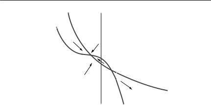
Fig. 8.3 Zero net growth isoclines for the competitive interaction between G. allenbyi and
G. pyramidum. The isoclines are shown in a state space of activity density for both species. The G. allenbyi isocline is the inverse sigmoid curve, and the G. pyramidum curve is approximately hyperbolic. A stable equilibrium is indicated by the converging arrows, whereas the other intersection of the isoclines represents an unstable equilibrium. From Abramsky et al. (1994).
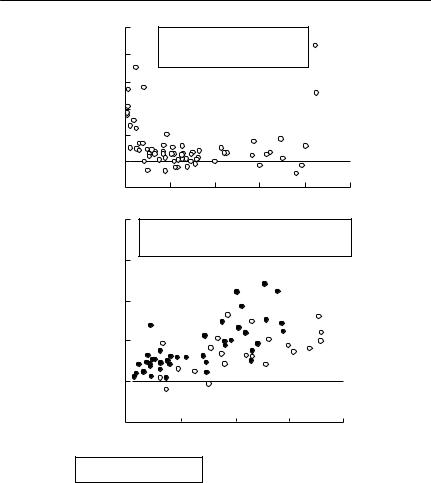
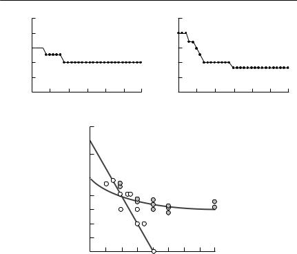
necessary. The targets were initially added at fairly high densities, which then declined towards a constant level over a period of a few days. The approximately constant level at which the target population ceased to decline was then taken to be the location of the zero isocline at that neighbour density (see Fig. 8.4(a)). The nonlinear isoclines thus obtained are shown in Fig. 8.4(b).
Whether these isoclines can be used to predict the outcome of competitive interactions between these two species in the field is doubtful. The competition investigated is only very short-term competition in a situation where emigration is prevented. No account is taken of either differing reproductive or dispersal ability. It is also difficult to see how such a method may be applied to species that are larger or disperse more widely or rapidly.
Estimating competition coefficients from census data
There has been a lengthy and continuing debate over whether competition coefficients can usefully be estimated from field data without some sort of manipulation (Crowell & Pimm, 1976; Pimm, 1985; Rosenzweig et al., 1985; Schoener, 1985; Pfister, 1995; Fox & Luo, 1996). Two main approaches have been suggested. The static approach uses data from a single snapshot recording of abundance of the two putative competitors at a number of sites, whereas the dynamic approach uses information on changes through time in the population size of the putative competitors.
M. per(no. sanguinipescage)
(a)
10
8
6

4
2
0 |
5 |
10 |
15 |
20 |
25 |
30 |
Time (days)
|
|
|
C O M P E T I T I O N |
231 |
||||
cage) |
10 |
|
|
|
|
|
|
|
8 |
|
|
|
|
|
|
||
per |
|
|
|
|
|
|
||
6 |
|
|
|
|
|
|
||
(no. |
|
|
|
|
|
|
||
4 |
|
|
|
|
|
|
||
T. kiowa |
|
|
|
|
|
|
||
2 |
|
|
|
|
|
|
||
0 |
5 |
10 |
15 |
20 |
25 |
30 |
||
|
||||||||
(b) |
|
|
Time (days) |
|
|
|||
M. sanguinipes (no. per cage)
(c)
9
8
7
6
5
4
3
2
1
0 |
1 |
2 |
3 |
4 |
5 |
6 |
7 |
8 |
T. kiowa (no. per cage)
Fig. 8.4 Derivation of nonlinear isoclines for competing grasshoppers. (a,b) Sample data from cages in which one grasshopper species (the agent) was held at a constant density in cages (by replacement of animals that died), whilst the other (the target) was allowed to decline without replacement. (a) shows Melanoplus sanguinipes as the target, and Trachyrachys kiowa as the agent. In (b) the target and agent are reversed. (c) The isoclines obtained by
a series of experiments similar to those shown above. The open circles represent data points where T. kiowa was the target, with the straight line passing through them being the estimated zero isocline for T. kiowa. The shaded circles represent data points where M. sanguinipes was the target. The nonlinear curve passing through them is the estimated
zero isocline for M. sanguinipes. The curve was assumed to be nonlinear a priori, based on a model of interspecific competition developed by Schoener (1974a) for species with exclusive, as well as shared, resources. From Chase (1996).
Static approaches
In principle, these methods are based on the reasonable idea that, if two species compete, there should be a negative correlation between the population densities at given sites, once confounding effects of habitat quality are removed. More formally, the zero-growth isocline for species N1 in a Lotka–Volterra model will be given by an equation of the following form:
N1 = K1 − α12N2. |
(8.10) |

232 C H A P T E R 8
Thus, if a series of sites can be found over which K2 varies, but α12 and K1 are constant, a regression of N1 versus N2 should have a slope of α12, provided the system is near equilibrium. There are a lot of provisos in this argument, sufficient that this very simple approach cannot be expected to work in practice.
The approach that has been used in practice was dubbed the ‘Pimm– Schoener’ method by Rosenzweig et al. (1985). The idea is to obtain data on the population density of the putative competitors at a number of sites and times, together with a range of variables describing the habitat from each of these observations. The objective is then to remove the confounding effects of habitat heterogeneity from the data statistically, so that the underlying relationship between the two species of interest is revealed. Using the population density of the ‘target’ species (or usually its logarithm) as a dependent variable, habitat variables are entered in a stepwise regression. The significance level for entry into the regression model would normally be set rather more loosely than the conventional p = 0.05, as environmental variation needs to be removed if it is possibly there. Following this, the density of the putative agent of competition is allowed to enter the regression, and the competition coefficient is then its regression parameter. The potential for measurement error bias in this approach is high.
Rosenzweig et al. (1985) used a number of variants of this method in a study of possible competition between desert rodents in Israel. The six variants were grouped into two subsets. In the first, principal components analysis was used to reduce the dimensionality of the habitat variables. Three subvariants were: (i) using a stepwise regression first, and then entering the census variables; (ii) using stepwise regression for habitat variables for both competitors, and then using regression on the residuals thus derived; and (iii) using a free regression, where census and habitat variables were entered together, with the order determined by the stepwise procedure itself. The second set used raw habitat descriptor variables instead of principal components, and then applied the three regression variants described above.
Their conclusion was that there was unacceptable inconsistency between methods, depending on the details of the method, although Pimm (1985) finds the consistency in the same analysis to be acceptable. There are certainly some statistical biases in using this approach. For example, the greater the ratio of the variance in the population size of the target of competition to the variance in population size of the agent, the larger is the estimated competition coefficient. This is simply because greater variation in density supplies more ‘support’ for a regression line. Without any extrinsic measure of competition, however, it is difficult to compare the various methods with any validity. Several studies have since compared the static regression approach with competition coefficients estimated from manipulations.
Abramsky et al. (1986) used two species of bumble-bee to compare the

C O M P E T I T I O N 233
regression model for detecting competition with direct manipulation of populations. Using a number of meadows that were separated by unsuitable habitat, the population size of each species was compared between control meadows with both species present and experimental meadows from which one or other of the species had been removed. The conclusion was that, whereas the manipulations detected competition, the regression model, based on only the unmanipulated meadows, could not. This conclusion is not really surprising. A complete removal is bound to be more powerful at detecting competition than is observation of the naturally existing range of densities.
Pfister (1995) conducted an elegant study of competition between fish in tidepools. She compared competition coefficients estimated by the Pimm– Schoener method with coefficients estimated by experimental manipulations, concluding that whereas the experimental manipulations provided strong evidence for competition, the regression analysis provided weak and inconsistent evidence. She suggested that part of the problem may have been that the carrying capacities for each pair of species were strongly correlated. This is what would be expected in tidepools, where volume is probably a dominant component of the carrying capacity. The regression method functions essentially by correcting for the carrying capacity of the target of competition, before examining the effect of the agent. If carrying capacities are strongly correlated, once this is done, there is very little signal left. Pfister (1995) also used a novel census-based approach, which used changes in population density through time, rather than simply population density, as the analysis variable. This approach appeared to work much more satisfactorily, and is described in the following section.
Fox and Luo (1996) have recently revisited the static regression approach, in a study comparing regression-based competition coefficients with estimates based on experimental removals. They examined competition between two Australian native rodents, Rattus lutreolus and Pseudomys gracilicaudatus, at four study sites in wet heathland. They suggest that the simple device of standardizing population densities before analysis (that is, subtracting the mean density from each observation, and then dividing by the standard deviation) will correct for the statistical artefact caused by differing variances. Experiments removing R. lutreolus were carried out at all four sites, to estimate the competition coefficient of R. lutreolus on P. gracilicaudatus. There was good agreement between these estimates and those based on regression using standardized data, but not with estimates based on raw densities.
Dynamic methods
Dynamic methods are not based on experimental manipulations of population sizes, but use the way in which densities of the competing species change

234 C H A P T E R 8
through time to estimate competition coefficients. Recent advances in statistical methods for the analysis of nonlinear time series have made this approach possible, and we can expect further developments and applications of this approach in the future. At present, few applications have appeared in the ecological literature.
Pfister (1995) based her method on a discrete-time version of the Lotka– Volterra model:
N (t |
+1) |
= r[K |
− N (t) − α |
|
|
|
|
||
ln |
1 |
|
|
12 |
N (t)]/K . |
(8.11) |
|||
|
|
||||||||
|
N1(t) |
|
1 |
1 |
2 |
1 |
|
||
|
|
|
|
|
|
||||
Here, all parameters and variables are as defined in eqn (8.1), except that N1(t + 1) and N1(t) represent the population size of N1 in successive time intervals. In principle, given a time series of N1 and N2, it is possible to fit this equation, estimating the parameter combinations r/K1, 1/K1 and α12/K1 using methods described by Dennis and Taper (1994) (see Chapter 6). Pfister (1995) estimated the parameters of eqn (8.11) using a time series over five censuses and five unmanipulated tidepools for the two most common fish species (Oligocottus maculosus and Clinocottus globiceps). The statistical method was a straightforward multiple regression with ln[N1(t + 1)/N1(t)] as the response variable, and N1(t) and N2(t) as the predictor variables. The only difficulty was that, because of the autoregressive structure of eqn (8.11), the usual standard errors, F tests, etc. could not be used. Pfister used a parametric bootstrap to assess the significance of the results (see Chapter 6 for details). She used all five replicate tidepools in a single analysis, yielding 20 data points. The results are shown in Table 8.1. They suggest that O. maculosus biomass has a significant negative effect on the change in C. globiceps biomass, but that there is no evidence of a reciprocal effect, nor of any effects on density. The only significant interspecific competitive interaction detected by removal experiments was that the growth of C. globiceps individuals was greater in pools from which O. maculosus had been removed, supporting the results of the dynamic regression. No significant interspecific interactions were detected by any of several variants of the static regression method applied to the same data.
Pascual and Kareiva (1996) used a more elaborate version of the dynamic approach to estimate parameters of a Lotka–Volterra model applied to Gause’s classic Paramecium data. Rather than using a simple difference-equation version of the Lotka–Volterra equations, they retained the original differential equation form, using the Runge–Kutta method (a standard numerical integration method) to integrate the equations numerically between the times of observation. This complicates the numerical calculations considerably, as standard statistical packages can no longer be used. In principle, however, the process is the same as Pfister’s approach.

C O M P E T I T I O N 235
Table 8.1 Results of dynamic regression models for tidepool fish. The table shows the results of dynamic regression models using eqn (8.11) on data from five replicate tidepools over four time intervals. The variable N1 represents either the numbers or the biomass
of the fish Oligocottus maculosus, and N2 represents either the numbers or biomass of the fish Clinocottus globiceps. Asterisks represent significance based on conventional multiple regression tests (*p < 0.05; **p < 0.01; ***p < 0.001). As is explained in the text, the autoregressive nature of the data means that these significance levels may be unreliable. The numbers in brackets are significance levels obtained from a bootstrap based on 1000 simulations (see text for details). Notice that the bootstrap results are much less significant than those based on multiple regression, which shows that conventional regression results may be quite misleading. The table also shows the overall R2 from the multiple regression.
This cannot be interpreted in a hypothesis-testing framework, but does show that the model based on biomass explained more variation than the one based on numbers. The overall interpretation of these results is that there is strong evidence of intraspecific competition
in both species, particularly when biomass is used as the variable, but that the only interspecific effect detectable is a negative impact of O. maculosus biomass on the change in C. globiceps biomass. Modified from Pfister (1995)
|
|
Independent variables |
|
|||
|
|
|
|
|
|
|
Dependent variable |
|
N |
(t) |
N |
(t) |
R2 |
|
1 |
|
2 |
|
|
|
|
|
|
|
|
|
|
Variables expressed as numbers per tidepool: |
|
|
|
|
|
|
ln(N1(t + 1)/N1(t)) |
− 0.718* |
− 0.153 |
0.261 |
|||
|
(0.35) |
|
|
|
||
ln(N2(t + 1)/N2(t)) |
− 0.061 |
− 0.364** |
0.338 |
|||
|
|
|
|
(0.028) |
|
|
Variables expressed as mass (g): |
|
|
|
|
|
|
ln(N1(t + 1)/N1(t)) |
− 0.909*** |
0.070 |
0.624 |
|||
|
(0.025) |
|
|
|
||
ln(N2(t + 1)/N2(t)) |
− 0.425** |
− 0.285*** |
0.597 |
|||
|
(0.041) |
(0.020) |
|
|||
|
|
|
|
|
|
|
The nature of the errors in the data is a critical factor that determines the appropriate method of parameter estimation. As I discuss in Chapter 2, ecological time-series data will include two forms of error. Process error is uncertainty about the actual value of N1(t + 1), given known values of N1(t) and N2(t). It is generated by such things as environmental variability and demographic stochasticity. Observation error occurs because the recorded value of N1(t + 1) is not the actual value of N1(t + 1), due to sampling error. Gause’s data could be expected to include both sources of error, but parameter estimation with both acting simultaneously is very difficult, especially if the relative size of the errors is not known a priori. Pascual and Kareiva (1996) took the approach suggested by Hilborn and Walters (1992) of running the estimation procedure assuming first, only process error, and second, only observation error. They then compared the results.
Assuming only process error, they proceeded as follows. For given estimates

236 C H A P T E R 8
of the parameters and starting populations N1(t) and N2(t), they predicted the values of N1(t + 1) and N2(t + 1) by integrating eqns (8.1) and (8.2). When they had done this over all the time intervals in the data for one set of parameter estimates, they repeated the process with another set of parameters. Finally, they selected the set of parameter estimates that minimized the discrepancy between the observed and predicted population changes. This ‘one-step-ahead’ prediction method is necessary for process error because the error accumulates: the starting point of the system for the next time step depends on the error in the previous step. However, it is assumed that the actual starting points for each step are known exactly.
If all the error is observation error, the fitting process is more similar to a conventional regression. For given estimates of the starting conditions and a set of parameter estimates, Pascual and Kareiva used the Runge–Kutta method to integrate an entire pair of trajectories. They then measured the discrepancy between the observed and predicted data points, and chose the set of parameters and starting points that minimized this discrepancy. This method is appropriate because the observation error model assumes that the error is in the eye of the beholder. The underlying process continues deterministically, given a set of starting values and parameter estimates, and an observation error at one time has no impact whatsoever on the future trajectory.
An important issue that they needed to resolve was how to measure the ‘discrepancy’ between observed and predicted values. The most appropriate method is maximum likelihood (see Chapter 2). This requires some assumption to be made about the probability distribution of the errors. Pascual and Kareiva assumed that it followed a lognormal distribution, both for process and for observation errors.
Table 8.2 shows the parameter estimates resulting from assuming either pure observation or pure process errors, and Fig. 8.5 shows the best fit of an observation error model. There is a reasonable degree of consistency in these results: both methods suggest that competition is asymmetrical, with the effect of P. aurelia on P. caudatum being much greater than the reverse effect. However, the best point estimates assuming only process error predict that P. aurelia should always win, whereas the best estimates assuming only observation error predict that the outcome should depend on the initial conditions (see Box 8.1).
Dynamic methods offer a powerful means of estimating interaction coefficients from census data. Their most important drawback, aside from the computational complexity, is that the model must be specified correctly. For Gause’s experiments, the simple Lotka–Volterra model without time delays, age structure, etc. can probably be justified. In longer-lived species with substantial maturation times and complex social behaviour, living in seasonal environments, the basic Lotka–Volterra model is unlikely to be a good
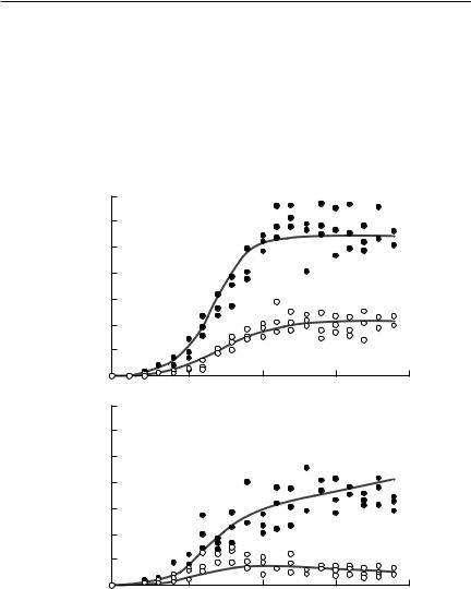
Table 8.2 Maximum likelihood estimates for the Lotka–Volterra model, fitted to Gause’s Paramecium data. The table shows maximum likelihood parameter estimates (MLEs), together with 95% confidence intervals. The parameters were fitted assuming either only observation error (columns 2 and 3) or only process error (columns 4 and 5). Subscripts on the parameters identify the species: Paramecium aurelia (species 1) and Paramecium caudatum (species 2). From Pascual and Kareiva (1996) (note, however, that the species identifications were reversed in this paper)
|
Observation error fit |
|
Process error fit |
|
|
|
|
|
|
|
|
Parameter |
MLE |
95% CI |
|
MLE |
95% CI |
|
|||||
|
|
|
|
|
|
r1 |
0.82 |
0.79–0.86 |
0.85 |
0.68–1.02 |
|
K1 |
5380 |
4820–6000 |
4920 |
4180–5900 |
|
α12 |
2.83 |
1.95–3.82 |
1.79 |
0.60–3.14 |
|
r2 |
0.63 |
0.60–0.66 |
0.64 |
0.48–0.79 |
|
K2 |
2000 |
1770–2280 |
1890 |
1520–2430 |
|
α21 |
0.46 |
0.36–0.56 |
0.40 |
0.25–0.61 |
|
σ 2 |
0.11 |
|
0.10 |
|
|
|
|
|
|
|
|
Density (no. per 5 cm3)
(a)
Density (no. per 5 cm3)
(b)
7000
6000
5000
4000
3000
2000
1000
0
7000
6000
5000
4000
3000
2000
1000
0
5 |
10 |
15 |
20 |
5 |
10 |
15 |
20 |
|
Time (days) |
|
|
Fig. 8.5 The fit of a Lotka–Volterra model with observation error to Gause’s Paramecium data. Paramecium aurelia numbers are shown with solid circles, and P. caudatum numbers are shown as open circles. (a) shows the case of the two species grown in separate cultures, whereas (b) shows the case when they were in mixed culture. The lines show the results predicted using an observation error model. From Pascual and Kareiva (1996) (note, however, that the species identifications were reversed in this paper).
238 C H A P T E R 8
description of the underlying dynamics. Fitting an inappropriate model, albeit by a sophisticated method, produces meaningless results. Pascual and Kareiva (1996) point out, quite correctly, that their general approach can be applied using any dynamic model that can be written down explicitly. Nevertheless, identifying an appropriate model is an essential precursor to any fitting procedure. A criterion such as Akaike’s information criterion (see Chapter 2) may help in model selection, but is no substitute for grounding models in biological reality.
Mechanistic models of competition
As discussed in Chapter 1, it is absolutely essential to be clear on the purpose of any modelling exercise before proceeding. Parameter estimation for a model is rarely a goal in itself: it is usually only worthwhile if the parameterized model is useful either for prediction or understanding of a particular sort of ecological interaction. The most likely use of a parameterized model of competition is to predict the outcome of a competitive interaction. Here, as Tilman (1990) has pointed out, many of the above methods become rather circular. The only entirely satisfactory way to estimate competition coefficients directly is via experiments in which the outcome of competitive interactions is observed. Thus, we need the answer to the question our model is intended to address before we can proceed with the model. Furthermore, Tilman (1990) points out that the experiments would rapidly become unworkable if questions about competitive interactions in even fairly small communities are addressed. If there are y species, (y2 + y)/2 pairwise series of experiments would be required.
The Lotka–Volterra model and its variants discussed above make no attempt to model explicitly the processes involved in competition. The Lotka–Volterra model itself subsumes the entire process of competition into the competition coefficients. Schoener (1974a) developed a model based on the proposition that there are both shared and exclusive resources, but the resources had no dynamics. An alternative approach, championed by Tilman (1982; 1987; 1990), is to recognize explicitly that resource competition involves interactions between the two or more potential competitors and their shared resources.
Tilman has applied his method primarily to plants and unicellular organisms, in which the situation is rather simpler than it is for animals, because the number of resources available to be shared is far smaller, but the approach is worth discussing in a book primarily directed towards animal ecology, as it offers the prospect of usefully predictive models. The principal limitation of the approach is that it is quite explicitly a means of looking at resource
Growth rate (dN/Ndt)
1.0
0.8
0.6
0.4
0.2
C O M P E T I T I O N 239
S.ulna
A. formosa
0 |
10 |
20 |
30 |
40 |
|
|
Resource (μM silicate) |
|
|
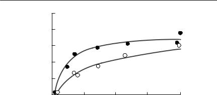
Fig. 8.6 Population growth of diatoms as a function of silicate concentration. These curves show the dependence of the per capita reproductive rate of the diatoms Synedra ulna and Asterionella formosa on silicate concentration at 24˚C. From Tilman (1982, p. 50).
competition, and will not assist with understanding or predicting the outcome of interference competition.
The simplest version of the model is as follows. Suppose the population size of competitor i is represented Ni, and that there is a single resource R. Then
|
dN |
= f (R) − m |
(8.12) |
|
|
N dt |
|||
|
|
|
||
and |
|
|
||
|
dR |
= y(R) − ∑Q N f (R). |
(8.13) |
|
|
|
|||
|
dt |
|
|
|
Here, fi(R) is the per capita growth rate of the population of competitor i, as a function of the resource level R; mi is the per capita death rate of i; and y(R) is the replenishment rate of the resource. The final term in eqn (8.13) describes the resource consumption by all the competitors. Tilman assumes that it is the product of the total growth rate of each competitor, multiplied by a competitor-specific proportionality constant Qi.
In simple cases, the functions fi(R) and y(R) can be measured experimentally. For example, Fig. 8.6 shows the growth rate of two species of diatom as a function of silicate concentration. It may also be possible to measure y(R) and Qi experimentally.
The main prediction of eqns (8.12) and (8.13) is that, following the competitive exclusion principle, one species will displace the others. The one that will do so is the competitor that reaches equilibrium with the lowest concentration
240 C H A P T E R 8
density ml) |
105 |
|
104 |
||
Population per(cells |
||
103 |
||
|
||
|
102 |
30 |
|
Af |
|
20 )M |
|
|
(μ |
10 |
Silicate |
|
|
101 |
10 |
20 |
30 |
40 |
50 |
0 |
0 |
|
(a)Time (days)
105 |
30 |
Population density (cells per ml)
104
103 


102
Su
20 |
(μM) |
|
|
10 |
Silicate |
|
Af
101 |
10 |
20 |
30 |
40 |
50 |
0 |
0 |
|
(c)Time (days)
density ml) |
105 |
|
104 |
||
Population per(cells |
||
103 |
||
|
||
|
102 |
Populationdensity per(cellsml) |
105 |
|
|
|
|
|
30 |
104 |
|
|
|
|
|
Silicate(μM) |
|
|
|
|
|
|
|
|
20 |
|
103 |
|
|
|
|
Su |
|
|
102 |
|
|
|
|
|
10 |
|
|
|
|
|
|
|
|
|
101 |
10 |
20 |
30 |
40 |
50 |
0 |
|
0 |
|
(b)Time (days)
Populationdensity per(cellsml) |
105 |
|
|
|
|
|
30 |
104 |
|
|
|
|
Su |
Silicate(μM) |
|
|
|
|
|
|
|
|
20 |
|
103 |
|
|
|
|
|
|
|
102 |
|
|
|
|
Af |
10 |
|
|
|
|
|
|
||
|
|
|
|
|
|
|
|
|
101 |
10 |
20 |
30 |
40 |
50 |
0 |
|
0 |
|
(d)Time (days)
30
Su |
(μM) |
|
20 |
||
|
||
10 |
Silicate |
|
|
Af
101 |
10 |
20 |
30 |
40 |
50 |
0 |
0 |
|
(e)Time (days)
Fig. 8.7 The outcome of competition experiments between diatoms. (a) The population density of the diatom Asterionella formosa (Af) growing by itself, and the concentration of silicate, the limiting nutrient, in the same flask (small dots) at 24˚C. (b) The population density of the diatom Synedra ulna (Su), also growing by itself and the concentration of silicate (small dots) at 24˚C. (c–e) Competition between the two diatoms, with three initial starting densities at 24˚C. In each case Synedra outcompetes Asterionella. From Tilman (1982, p. 52).
of the resource, R*, when grown in monoculture. Some experimental results obtained by Tilman supporting this prediction are shown in Fig. 8.7.
In principle, this idea can readily be generalized to a number of resources (Tilman, 1982). Suppose that there are n competitors, that the population size of competitor i is represented by Ni, and that there are k resources Rj. Then

|
|
|
|
|
|
|
|
|
|
|
C O M P E T I T I O N 241 |
|
dN |
= f |
(R1,R2 ,... ,Rk ) − m |
|
|
|
|
(8.14) |
|||
|
|
|
|
|
|
|
|||||
|
N dt |
|
|
|
|
||||||
|
|
|
|
|
|
|
|
|
|
||
and |
|
|
|
|
|
|
|
|
|
||
|
dRj |
= y |
(R |
) − ∑N f (R |
,R |
,... ,R )q |
(R |
,R |
,... ,R ). |
|
|
|
|
(8.15) |
|||||||||
|
dt |
j |
j |
1 |
2 |
k j |
1 |
2 |
k |
||
|
|
|
|
|
|
|
|
|
|||
Here fi is a function describing the dependence of the rate of growth of species i on the availability of the resources Rj, and qij is the generalization of Qi, describing how the consumption rate of each resource depends on the growth rate of each competitor.
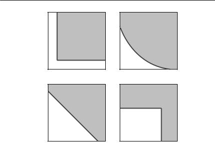
The outcome of an interaction described by eqns (8.14) and (8.15) depends on the form of the functions fi(R1, . . . ,Rk), which describe how the growth rate of each species depends on the level of each resource. Tilman (1982) developed a powerful graphical technique to predict the outcome. For each competitor, a zero net growth isocline can be constructed as a function of resource concentration. Figure 8.8 shows some forms that these isoclines might take if there are two resources. Tilman experimentally obtained such isoclines for several species of diatoms, and showed that he could successfully predict the outcome of competition in ‘chemostat’ experiments, in which resources were supplied at a constant rate.
This general approach offers the prospect of genuinely predictive models of resource competition. The challenge that remains is to apply the models to multicellular animals in heterogeneous environments, rather than to unicellular organisms or plants.
Summary and recommendations
1 Resource overlap indices are exactly that and no more: they cannot be used to infer either the existence of or extent of competition.
2 If a pair of interacting species is embedded in a larger community (and this is almost always the case), indirect effects may mean that the overall effect on one species of perturbing the population size of another may be quite different from the effect expected from the direct interaction coefficient.
3 Manipulative experiments offer the best prospect of estimating the strength of a competitive interaction. As with any ecological experiment, adequate replication and appropriate controls are essential. It is equally important that the experimental setup should be reasonably representative of the natural situation, and that the spatial and temporal scales of the experiment should be appropriate.
4 Removal experiments are the most straightforward way to estimate competition coefficients. In such experiments, the population size of a target
242 C H A P T E R 8
2 |
|
2 |
or S |
|
or S |
2 |
|
2 |
R |
|
R |
(a) |
R1 or S1 |
(b) |
2 |
|
2 |
or S |
|
or S |
2 |
|
2 |
R |
|
R |
(c) |
R1 or S1 |
(d) |
R1 or S1
R1 or S1
Fig. 8.8 Some possible forms of zero net growth isoclines with two resources. In each of these graphs, the concentration of two resources is shown on the two axes. The zero net growth isocline for a consumer is shown as a solid line. In the shaded region the consumer’s population can increase, whereas in the unshaded region insufficient resources are available for growth. (a) Essential resources. Each resource is needed for growth, so minimum levels of resources 1 and 2 must both be available to the consumer. (b) Complementary resources. Neither resource is absolutely essential, but the growth rate is higher if both are consumed together than would be predicted by simply adding the growth rates expected from consuming either resource alone. The zero net growth isocline is therefore bowed in towards the origin, if both resources are available. (c) Substitutable resources. Each resource can replace the other, so the growth rate is determined by the resource concentrations added together. (d) Switching resources. The consumer can use either resource, so that minimum levels of resource 1 or resource 2 must be available to the consumer. From Tilman (1982, p. 62).
species is compared between experimental units that are intact, and units where the putative agent of competition has been removed. The interaction coefficients estimated by removal experiments include indirect as well as direct effects. They characterize the competitive interaction completely only if the isoclines are linear.
5 Pulse experiments are theoretically the best way to measure direct interaction coefficients in complex communities. In such experiments, individual species are perturbed one at a time, and the response of the population growth rate of all species to the perturbation is recorded. They are, however, logistically difficult in practice, and have rarely been used.
6 In the few cases that have been looked at systematically, competitive isoclines have been found to be nonlinear. This means that the interaction cannot adequately be characterized by a single competition coefficient.

C O M P E T I T I O N 243
7 Purely observational methods may give an indication of whether competition is occurring, particularly if time-series data are used, but are unlikely to provide sufficient information to develop a predictive model of a competitive interaction.
8 Models based on explicit resource dynamics offer the best prospect of producing predictive models of competitive interactions. Their potential, however, has yet to be fully realized.