


C H A P T E R 5
Rate of increase of a population
Introduction
The rate of increase of a population is a parameter basic to a great many ecological models. It is, however, an abstract quantity, being a combination and summary of age-specific mortality and fecundity. Perhaps more than any other parameter, the value appropriate for use in a model is context-dependent, varying both with the structure of the model and the model’s purpose. In broad terms, estimates of r are required in two sorts of models: deterministic models, often of interspecific interactions or harvesting; and stochastic models, often used for population viability analysis of single species. Most deterministic models aim for a qualitative and general representation of population behaviour so that statistically rigorous estimation methods are not necessary. The main problem is to ensure that the rate being estimated is appropriate to the context of the model. Stochastic models, usually of single species, are likely to be directed at answering quantitative questions about specific populations and will thus require estimates that are as accurate as possible.
Definitions
The rate of increase r is defined from the most basic of population models, that for exponential growth,
|
dN |
= rN , |
(5.1) |
|
|
||
|
dt |
|
|
with the solution |
|
||
N(t) = N(0)ert. |
(5.2) |
||
Following this definition, r is an empirical quantity, and can be estimated from a time series of population size and time, without any need to consider the processes underlying population growth or decline.
In most deterministic models, however, the appropriate value of r is the maximum rate of population growth possible for the given species in the particular environment, excluding density-dependent constraints and any other factors that are explicitly included in the model. This quantity is often called rmax or rm (for example, Caughley, 1977a) and referred to as the intrinsic rate of increase. An important point about this definition is that rmax is a property
139

140 C H A P T E R 5
of both the species and the environment the particular population inhabits. It is not a characteristic of the species alone.
Caughley (1977a) also defines two other rates of increase. These are rS, the rate of increase at which a population would increase given the current fecundity and mortality schedules, once a stable age distribution is reached, and W, the observed rate of increase of a particular population over a particular time period. Caughley’s notation is useful, eliminating potential sources of confusion, but has not entered general usage. Most authors simply use r, and which of the different rates actually being referred to must be determined from the context.
In most circumstances, deriving r from a simple time series of population size will underestimate rmax, as various density-dependent factors are likely to be acting. The exception is when the population is increasing from a low base, in which case an estimate derived from a time series may well be appropriate.
The finite rate of increase λt is the proportional increase in total population size over a specified time interval (t, t + t), i.e.
λt = |
Nt+Δt |
|
(5.3) |
|
Nt |
||||
|
|
|||
or |
|
|
|
|
ln(λt) = ln(Nt+Δt) − ln(Nt). |
(5.4) |
|||
Assuming that r has remained constant over the time interval |
t, λ and r are |
|||
related by the simple equation |
|
|||
ln(λt) = r t. |
(5.5) |
|||
Estimating r from life-history information
The Euler–Lotka equation
Given a set of age-specific fecundities and mortalities, the potential rate of increase of a population can be determined from the solution of the Euler–Lotka equation:
∞ |
|
|
|
∑e−rxF l |
x |
= 1. |
(5.6) |
x |
|
|
x=1
Here, x is the age of individuals, lx is the age-specific survivorship (the proportion of individuals surviving from the first census to age x), and Fx is the age-specific fertility, or the number of individuals entering the first year class per individual of age x.

R A T E O F I N C R E A S E O F A P O P U L A T I O N 141
Defining parameters for the Euler–Lotka equation
There is considerable confusion in the literature concerning correct definitions of the parameters for the Euler–Lotka equation, and several textbooks are in error (Jenkins, 1988). To avoid these problems, a good solution is to index the age classes from x = 1, rather than from x = 0, that is, call the first age class age 1, not age 0. If this is done, it is best also to define lx as the proportion of individuals surviving from the first census to age x, not from birth to age x as many authors do. Finally, it necessary to be very careful with the definition of age-specific fertility. In general, the number of newborn females produced per female of age x per unit of time (often called mx) is not the appropriate definition of Fx required.
The difficulty arises because Fx is the number of individuals born since the previous census, alive at the current census, per individual of age class x present at the previous census. This means that the timing of the census relative to the timing of reproduction is important. Caswell (1989) has a particularly good discussion of the problems involved. You need first to decide whether your population breeds continuously (a birth-flow population) or whether births occur in a short, well-defined breeding season (a birth-pulse population).
In a birth-flow population, newborns will, on average, have to survive half a census interval to be counted in the first census and not all individuals of a particular age present at the previous census will survive long enough to give birth. Defining Px as the probability that an individual will survive from age x to age x + 1, and PJ/2 as the probability of a newborn surviving half the interval between censuses, Caswell shows that
F = P |
m |
x |
+ P m |
x+1 |
|
|
|
|
|
x |
. |
(5.7) |
|||
|
|
2 |
|
||||
x J/2 |
|
|
|
|
|
||
The formal derivation of eqn (5.7) is given in Caswell (1989). The first term is straightforward to understand: on average, newborns must survive half a census interval to be counted. The second term is trickier. The easiest way to understand it intuitively is that it is the average of mx, the fecundity of individuals of age class x immediately after one census (when they are all still alive) and the reproductive output immediately before the next census when only the proportion Px of the age class remains alive, but their fecundity is mx+1.
In principle, birth-pulse populations could be censused at any time relative to the breeding season. It is convenient, however, to restrict discussion to either of two extremes: a census immediately preceding breeding, or a census immediately following breeding. For a prebreeding census, juveniles will only be counted if they have survived the entire census interval, but all individuals in age class x in the previous census will have survived to be able to breed. Thus

142 C H A P T E R 5 |
|
Fx = mx PJ, |
(5.8) |
where PJ is the survival rate of juveniles in their first census interval. Conversely, for a post-breeding census, all juveniles born since the previous census will survive to be counted, but only a proportion Px of individuals in age class x in the previous census will survive to reproduce. Hence
Fx = mx Px. |
(5.9) |
The problem of estimating survival and fecundity is considered in Chapter 4.
Solving the equation
The Euler–Lotka equation is an implicit equation for r. This means that (except for particular functional forms of lx and Fx), it cannot be manipulated into a form r = f(lx, Fx). It must instead be solved by a process of successive approximation, in which the value of r is varied until the left-hand side of the equation equals 1. This is very easy to do using most spreadsheets (see Box 5.1). The r estimated is rS: the rate at which the population would grow once a stable age distribution is reached.
Cole (1954) derived the following approximate form of the Euler–Lotka equation:
1 = e−r + be−ra − be−r(m+1), |
(5.10) |
Box 5.1 Using a spreadsheet to solve the Euler–Lotka equation
This example uses the schedules shown in Table 5.1, and Excel notation. Step 1. Enter age, fecundity and survival schedules:
|
|
|
|
|
|
|
|
|
|
|
|
|
|
A |
B |
C |
D |
E |
F |
G |
H |
I |
|
|
|
|
|
|
|
|
|
|
|
|
|
|
1 |
Age |
1 |
2 |
3 |
4 |
5 |
6 |
7 |
8 |
|
|
2 |
Fx |
0 |
0.25 |
0.4 |
0.8 |
0.8 |
0.6 |
0.5 |
0.2 |
|
|
3 |
Px |
0.5 |
0.8 |
0.9 |
0.9 |
0.9 |
0.8 |
0.7 |
0 |
|
|
|
|
|
|
|
|
|
|
|
|
|
|
|
|
|
|
|
|
|
|
|
|
|
Step 2. Enter formulae to calculate lx for ages 1 and 2 into cells B4 and C4 and for e−rxlx Fx for age 1 into cell B5. Note that $J$2 ensures that cell J2 is referenced even when the formula is copied to other columns. A trial value of r is placed in cell J2.
continued on p. 143

R A T E O F I N C R E A S E O F A P O P U L A T I O N 143
Box 5.1 contd
|
|
A |
|
B |
|
C |
|
D |
|
E |
|
F |
|
G |
|
H |
|
I |
|
J |
|
|
|
|
|
|
|
|
|
|
|
||||||||||
|
|
|
|
|
|
|
|
|
|
|
|
|
|
|
|
|
|
|
|
|
|
1 |
Age |
|
1 |
|
2 |
|
3 |
|
4 |
|
5 |
|
6 |
|
7 |
|
8 |
|
r |
|
2 |
Fx |
|
0 |
|
0.25 |
|
0.4 |
|
0.8 |
|
0.8 |
|
0.6 |
|
0.5 |
|
0.2 |
|
0.05 |
|
3 |
Px |
|
0.5 |
|
0.8 |
|
0.9 |
|
0.9 |
|
0.9 |
|
0.8 |
|
0.7 |
|
0 |
|
|
|
4 |
lx |
|
|
|
|
|
|
|
|
|
|
|
|
|
|
|
|
|
|
|
|
1 |
|
= B4*B3 |
|
|
|
|
|
|
|
|
|
|
|
|
||||
|
5 |
exp |
|
|
|
|
|
|
|
|
|
|
|
|
|
|
|
|
|
|
|
|
= exp(–B1*$J$2)*B4*B2 |
|
|
|
|
|
|
|
|
|
|
||||||||
|
|
|
|
|
|
|
|
|
|
|
|
|
|
|
|
|
|
|
|
|
|
|
|
|
|
|
|
|
|
|
|
|
|
|
|
|
|
|
|
|
|
Step 3. Copy these across the other ages and sum row 5 in cell J5.
|
|
|
|
|
|
|
|
|
|
|
|
|
|
|
|
|
|
A |
B |
C |
D |
E |
F |
G |
H |
I |
J |
K |
|
L |
|
|
|
|
|
|
|
|
|
|
|
|
|
|
|
|
|
|
1 |
Age |
1 |
2 |
3 |
4 |
5 |
6 |
7 |
8 |
r |
|
|
|
|
|
2 |
Fx |
0 |
0.25 |
0.4 |
0.8 |
0.8 |
0.6 |
0.5 |
0.2 |
0.05 |
|
|
|
|
|
3 |
Px |
0.5 |
0.8 |
0.9 |
0.9 |
0.9 |
0.8 |
0.7 |
0 |
|
|
|
|
|
|
4 |
lx |
1 |
0.5 |
0.4 |
0.36 |
0.32 |
0.29 |
0.23 |
0.16 |
|
|
|
|
|
|
5 |
|
|
|
|
|
|
|
|
|
|
|
|
|
|
|
exp |
0 |
0.11 |
0.14 |
0.24 |
0.2 |
0.13 |
0.08 |
0.02 |
=Sum(B5:15) |
|
|
|||
|
|
|
|
|
|
|
|
|
|
|
|
|
|
|
|
|
|
|
|
|
|
|
|
|
|
|
|
|
|
|
|
Step 4. Use ‘Goal Seek’ to set cell J5 to 1 by altering cell J2.
‘Goal Seek’ is an Excel feature that uses successive approximations to set a certain cell in the spreadsheet to a specified value by altering the value of a number in another cell of the spreadsheet. It needs to be given an initial guess of the value of r to commence the process.
|
|
|
|
|
|
|
|
|
|
|
|
|
|
|
|
|
A |
B |
C |
D |
E |
F |
G |
H |
I |
J |
K |
L |
|
|
|
|
|
|
|
|
|
|
|
|
|
|
|
|
|
1 |
Age |
1 |
2 |
3 |
4 |
5 |
6 |
7 |
8 |
r |
|
|
|
|
2 |
Fx |
0 |
0.25 |
0.4 |
0.8 |
0.8 |
0.6 |
0.5 |
0.2 |
0.03 |
|
|
|
|
3 |
Px |
0.5 |
0.8 |
0.9 |
0.9 |
0.9 |
0.8 |
0.7 |
0 |
|
|
|
|
|
4 |
lx |
1 |
0.5 |
0.4 |
0.36 |
0.32 |
0.29 |
0.23 |
0.16 |
|
|
|
|
|
5 |
exp |
0 |
0.11 |
0.14 |
0.24 |
0.2 |
0.13 |
0.08 |
0.02 |
1 |
|
|
|
|
|
|
|
|||||||||||
|
|
|
|
|
|
|
|
|
|
|
|
|
|
|
|
|
|
|
|
|
|
|
|
|
|
|
|
|
|

144 |
C H A P T E R 5 |
|
|
|
|
|
|
|
Table 5.1 A hypothetical fertility and survivorship schedule |
|
|
|
|||||
|
|
|
|
|
|
|
|
|
Age |
1 |
2 |
3 |
4 |
5 |
6 |
7 |
8 |
|
|
|
|
|
|
|
|
|
Fx |
0 |
0.25 |
0.4 |
0.8 |
0.8 |
0.6 |
0.5 |
0.2 |
Px |
0.5 |
0.8 |
0.9 |
0.9 |
0.9 |
0.8 |
0.7 |
0 |
|
|
|
|
|
|
|
|
|
where b is the average number of offspring produced, a is the age at first reproduction and m is the age at last reproduction. Cole’s equation assumes that reproduction occurs once per time interval, and that all females survive until after age m. It has been used in at least two recent studies (Hennemann, 1983; Thompson, 1987), but will always overestimate r because of the simple step function assumed for survivorship. Given the ease with which the Euler– Lotka equation can be solved on spreadsheets, there is now little need for approximate forms.
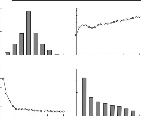
Depending on the shape of the initial age distribution, rS may be very different from the r calculated by applying eqn (5.5) to a few years of growth in total population size. Consider the hypothetical fertility and survivorship schedules in Table 5.1, chosen to represent a population of macropods in good conditions immediately following the breaking of a drought. The value of rS predicted from this schedule using eqn (5.6) is rS = 0.032 0. Just before a drought breaks, it is likely that there will be very few juveniles in the population, and the age distribution might resemble that shown in Fig. 5.1(a). Figure 5.1(b) shows the total population size projected from this initial age distribution using the schedules in Table 5.1, and Fig. 5.1(c) shows r calculated from applying eqn (5.5) from year 1 forward to each subsequent year. Finally, Fig. 5.1(d) shows the stable age distribution reached after 20 years.
It is obvious that, for the first few years, the population grows at an average rate much greater than that predicted by the Euler equation. In fact, in the first year, the growth rate is 10 times higher than rS. The reason in this particular case is that the initial age distribution contains a far higher proportion of animals in the age range of maximum fecundity than does the stable age distribution. One would expect a similar pattern in a translocation. It is usual to commence translocations with young adults, which will be individuals with particularly high survivorship and fecundity. Even without changes in the underlying age-specific survivorship and fecundity, one would not expect the initial rate of increase of a translocated population to be maintained.
Estimating rmax from the Euler–Lotka equation
Assuming that the parameters of the life table have been defined correctly, there is still the substantial problem of choosing estimates of these to estimate
|
|
|
|
|
|
|
|
|
|
R A T E O F I N C R E A S E O F A P O P U L A T I O N |
|
145 |
|||||||||
|
40 |
|
|
|
|
|
|
|
|
|
2000 |
|
|
|
|
|
|
|
|
|
|
|
30 |
|
|
|
|
|
|
|
|
|
size |
|
|
|
|
|
|
|
|
|
|
Percentage |
20 |
|
|
|
|
|
|
|
|
|
population |
|
|
|
|
|
|
|
|
|
|
|
|
|
|
|
|
|
|
|
|
|
|
|
|
|
|
|
|
|
|
|
|
|
10 |
|
|
|
|
|
|
|
|
|
Total |
|
|
|
|
|
|
|
|
|
|
|
|
|
|
|
|
|
|
|
|
|
|
|
|
|
|
|
|
|
|
|
|
|
0 |
|
|
|
|
|
|
|
|
|
|
200 |
|
|
|
|
|
|
|
|
|
|
1 |
2 |
3 |
4 |
5 |
6 |
7 |
8 |
9 |
|
0 |
|
5 |
|
|
10 |
|
15 |
|
20 |
|
|
|
|
|
|
|
|
|
||||||||||||||
(a) |
|
|
|
Age (years) |
|
|
|
|
(b) |
|
|
|
|
Time (years) |
|
|
|
|
|||
|
0.5 |
|
|
|
|
|
|
|
|
|
|
40 |
|
|
|
|
|
|
|
|
|
|
0.4 |
|
|
|
|
|
|
|
|
|
|
30 |
|
|
|
|
|
|
|
|
|
|
|
|
|
|
|
|
|
|
|
|
Percentage |
|
|
|
|
|
|
|
|
|
|
r |
0.3 |
|
|
|
|
|
|
|
|
|
|
|
|
|
|
|
|
|
|
|
|
|
|
|
|
|
|
|
|
|
|
|
|
|
|
|
|
|
|
|
|
|
|
|
|
|
|
|
|
|
|
|
|
|
|
20 |
|
|
|
|
|
|
|
|
|
|
0.2 |
|
|
|
|
|
|
|
|
|
|
|
|
|
|
|
|
|
|
|
|
|
0.1 |
|
|
|
|
|
|
|
|
|
|
10 |
|
|
|
|
|
|
|
|
|
|
|
|
|
|
|
|
|
|
|
|
|
|
|
|
|
|
|
|
|
|
|
|
0.0 |
|
|
|
|
|
|
|
|
|
|
0 |
|
|
|
|
|
|
|
|
|
|
0 |
|
5 |
|
|
10 |
|
15 |
|
20 |
|
1 |
2 |
3 |
4 |
5 |
6 |
7 |
8 |
9 |
|
|
|
|
|
|
|
|
|
||||||||||||||
(c) |
|
|
|
Time (years) |
|
|
|
|
(d) |
|
|
|
|
Age (years) |
|
|
|
|
|||
Fig. 5.1 The effect of the initial age distribution on the rate of population growth. Given the initial age distribution in (a), the fecundity and survivorship schedules in Table 5.1 will lead to the population growing as shown in (b). The estimated growth rate from time 0 to each time is shown in (c). The stable age distribution for these schedules is shown in (d). When this distribution is reached, the population will grow at the constant rate rS = 0.032 0.
rmax. Data from a field population will not be appropriate unless that population either is increasing at rmax, or at least would do so if current conditions continued long enough for a stable age distribution to be reached. Suitable values of mx can often be obtained from laboratory or captive populations: age at first breeding, gestation time, interval between breeding and litter or clutch size of captive populations are probably reasonable indications of what might be expected in the field under good conditions. As I discuss in the previous chapter, survival of captive animals gives a much poorer indication of survival in the wild. One possible approach is that used by Tanner (1975), who used the highest rates of juvenile and adult survival he could find in the literature to calculate rmax for 13 species of mammals. His estimates were, however, criticized by Caughley and Krebs (1983) as being too low. For example, Caughley and Krebs (1983) derive rmax for white-tailed deer as being at least 0.55 on the basis that an introduction of six animals had increased to 160 in six years,

146 C H A P T E R 5
whereas Tanner’s estimate is 0.30. The example in Fig. 5.1 cautions, however, that the initial rate of increase of a population of adult animals may greatly exceed rS for that same population and environment.
Estimating r for stage-structured populations
The population dynamics of many species can be better described by dividing the population into stages, which may be of differing or variable duration, rather than ages, where each age class has an equal and fixed duration. Stages may be distinct developmental stages (egg, larva, pupa, etc.) or may be size classes. The critical difference from age-structured populations is that surviving individuals do not necessarily progress into the next stage each time step, but may also remain in the same stage, possibly jump two or more steps forward, or even drop back one or more stages.
There is an outstanding discussion of stage-structured discrete models in Caswell (1989), which I will summarize very briefly here. In principle, r can be estimated by a straightforward generalization of the approaches used for agestructured models. A square projection matrix is constructed, the elements of which contain transition coefficients. For example, aij, the coefficient in the ith row and jth column, gives the number of individuals in stage i next time step, per individual in stage j at the previous time. Hence,
s |
|
n (t + 1) = ∑a jnj(t). |
(5.11) |
j=1
Having constructed the matrix, the long-term finite rate of increase, once a stable stage distribution is reached, is given by the dominant eigenvalue λ of the transition matrix. By rearranging eqn (5.5),
r = |
ln(λ) |
, |
(5.12) |
s |
t |
|
where t is the length of the time step. Various computer packages for mathematical analysis can extract eigenvalues from matrices – for example, Mathematica (Wolfram, 1991). Methods to calculate eigenvalues can also be found in Press et al. (1994). In general, an n × n matrix has n eigenvalues, and these are often complex numbers. The dominant eigenvalue is the one with the largest magnitude of the real part.
As with age-structured models, it is necessary to be careful about defining fecundity terms in the matrix, particularly with respect to the timing of reproduction relative to the timing of the census. The crucial point remains that the first row of the matrix must contain the number of members of the initial stage at the current census per individual of each stage present at the previous census.

R A T E O F I N C R E A S E O F A P O P U L A T I O N 147
Estimating r from time series
The most obvious way to estimate r from a time series is from the slope of a least squares linear regression of ln(N) versus t, as suggested, for example, by Caughley and Sinclair (1994). A simple linear regression in this situation is a rather dubious exercise, however, as the errors associated with successive data points are likely to be related (autocorrelated) because random variations in any given sampling occasion will probably influence population size over a number of subsequent samples. Whether or not this statistical problem matters depends on what the estimate is required for and the relative importance of sources of variation in the time series.
There are at least three sources of ‘error’ or variation in a series of population size values versus time. As is discussed in Chapter 2, there is observation error: most such data sets are a series of estimates of population size or density rather than complete enumerations of the population. There also is process error of two sorts: some is associated with the fact that population size is finite and must be a whole number. Equation (5.1) is a deterministic equation, whereas actual population growth will be stochastic, or random. Birth and death are discrete processes that either do or do not occur to particular individuals in a certain time interval with particular probabilities. This form of randomness is often called ‘demographic stochasticity’. The other source of process error is environmental stochasticity: temporal changes in the underlying rates of birth and death caused by environmental variability such as good or bad seasons.
There is no reason to expect observation errors in adjacent recording times to be related, unless the recording interval is so short that weather-related sightability or catchability influences more than one census. An exception may occur if population estimates are based on mark–resight or mark–recapture methods (see Chapter 3), although autocorrelation of such estimates does not seem to have formally been studied. If the population under study is large, it exists in a fairly constant environment and it is not subject to significant density dependence, then its population dynamics may be approximated well by eqn (5.1). In that case, variation in the estimated population size will predominantly be a result of sampling error, and a simple regression of ln(N) versus time will be the best way to estimate r.
In many (probably most) cases, there will be substantial variation in population size and population growth rate as a result of environmental stochasticity. This will introduce autocorrelation into the error terms of the time series, producing problems, particularly in the estimation of the standard error of the growth rate. A standard method in time-series analysis to reduce autocorrelation is to use differences between successive observations as the analysis variable. It is possible to show that this process will eliminate autocorrelation from a time series of population size generated from ageor stage-structured models
148 C H A P T E R 5
such as those described by eqn (5.11), provided the transition probabilities are not correlated (Dennis et al., 1991). In ecological terms, this means that age-dependent survival or fertility can vary according to environmental conditions, but such variation must be independent between observation periods.
If differences in log population size are calculated between observation periods with an initial population size observation N0, and n subsequent observations N1, . . . , Nn one time unit apart, then the mean growth rate can be estimated as
|
n |
|
N |
|
|
|
||
W = ∑ln |
|
n. |
(5.13) |
|||||
N |
|
|||||||
|
=1 |
|
−1 |
|
|
|
||
|
|
|
|
|
|
|||
This follows in a straightforward way from eqn (5.4). There are, however, complications. First, eqn (5.13) can easily be arranged into the form
W = [ln(Nn) − ln(N0)]/n, |
(5.14) |
meaning that the estimate of r is obtained only from the first and last values in the series. Intermediate values do not contribute at all to the point estimate, although they will influence its standard error. This is not unreasonable if the Ni are true counts, because both values are ones the population has in fact taken, and intermediate values have contributed to Nn in the sense that each population size builds on previous values. If the Ni are only estimates of population size, this estimation method has the undesirable feature that a single aberrant observation at the beginning or end will greatly effect the estimate of r. It is intriguing that this statistically rigorous approach produces the same point estimate as the very elementary approach that has been used by several authors (for example, Caughley & Krebs, 1983; Hanski & Korpimäki, 1995) of estimating r from two records only of population size over time.
A second difficulty is that eqns (5.13) and (5.14) measure the average growth rate of the population. This is not the same as the growth rate of the expected, or average, population size (Caswell, 1989). The difference is that the expected or average growth rate of a population is determined by the average of log population size, whereas the growth rate of the average population size is determined by the log of average population size. The growth rate of the average population size can be estimated by
? = W + |
& 2 |
. |
|
|
|
|
(5.15) |
|
2 |
|
|
|
|
||||
|
|
|
|
|
|
|
|
|
Here is &2 the sample variance of ln(N |
/N |
i−1 |
) (Dennis et al., 1991), given by |
|||||
|
|
|
|
|
i |
|
|
|
|
∑(r − |
|
) |
|
|
|
||
&2 = |
r |
|
|
(5.16) |
||||
|
, |
|
|
|||||
|
|
(n − 1) |
|
|
|
|||

R A T E O F I N C R E A S E O F A P O P U L A T I O N 149
where ri = ln(Ni/Ni−1).
If the interval between observations is not constant, the problem becomes more complex. Defining τi as the time interval between recording Ni−1 and Ni, Dennis et al. (1991) show that W and &2 can be estimated by a linear regression
without intercept between |
|
|||||
|
N |
i |
|
|
|
|
yi |
= ln |
|
|
τ i |
(5.17) |
|
|
|
|||||
|
Ni−1 |
|
|
|||
as the dependent variable and τ i as the independent variable. The slope of the relationship is W, and &2 is the mean square error for the regression. Provided n, the number of terms in the series, is not too small, ? is approximately normally distributed with standard error
se = |
& 2 |
|
1 |
+ |
& 2 |
|
|
|
|
|
, |
(5.18) |
|||
|
|
||||||
? |
|
tn |
|
2(n −1) |
|
||
|
|
|
|
||||
where tn is the length of the series in time units.
An example of the application of this method to the classic data set of reindeer population growth after their introduction to St Paul Island in the Bering Sea (Scheffer, 1951) is given in Box 5.2.
It should be emphasized that, strictly speaking, this approach is only applicable if population size is known exactly. The question of how best to analyse data when both environmental stochasticity and sampling error are important has not satisfactorily been answered, but the problem is considered in Barker and Sauer (1992) and Sauer et al. (1994). (Also see Chapter 11.)
Box 5.2 Analysis of the growth rate of the St Paul Island reindeer population
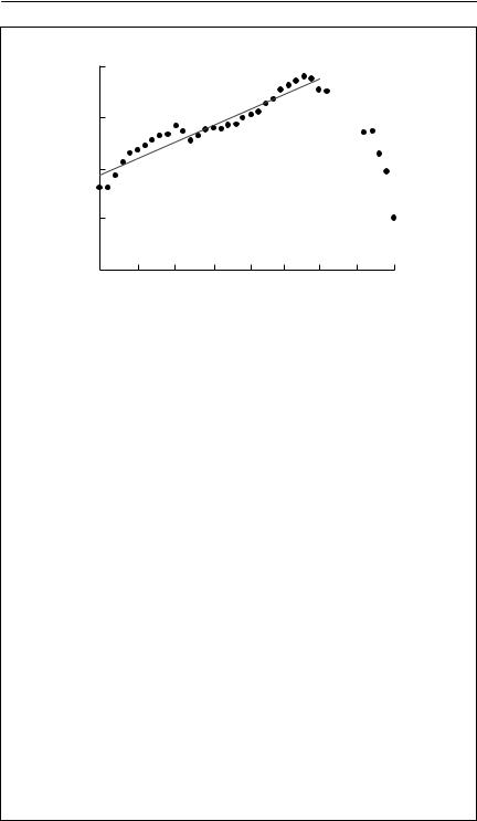
In 1911, four male and 21 female reindeer were introduced on to St Paul Island (106 km2) in the Bering Sea. By 1938, the population had increased to about 2000 animals in what has come to be regarded as a classic example of exponential population growth (Krebs, 1985). The population then crashed to eight animals in 1950. In this box, some of the methods of estimating r in Chapter 5 are applied to this data set using the data from 1911 through to 1940.
The original data are shown in the figure, plotted on a log scale with the least squares regression line from 1911 to 1940 superimposed. It appears that the residuals are highly autocorrelated, as there are long runs or values
continued on p. 150
150 C H A P T E R 5
Box 5.2 contd
ln(Nt)
8
6
4
2
0
1911 |
1916 |
1921 |
1926 |
1931 |
1935 |
1940 |
1945 |
1950 |
|
|
|
|
Year |
|
|
|
|
above and below the linear regression line. A standard way of testing for autocorrelation is to use a Durbin–Watson test (Kendall, 1976). The test statistic d is around 2 if a time series is not autocorrelated. The value of d obtained from analysis of ln(N ) versus time up to 1940 is 0.388, which is much smaller than the critical value at p = 0.01 of 1.13. The gradient of the relationship, which is often used as an estimate of r, is 0.130. The standard error of the estimated value of r will be an underestimate of the true standard error because of the autocorrelation. It is 0.007 1.
The alternative approach is to use Xt = ln(Nt /Nt−1) as the analysis variable. In this case, the data are still autocorrelated (d = 1.127, p = 0.01). The result suggests that there may be serial correlation in age-specific survival and mortality, as Dennis et al. (1991) have shown that Xt should be independent if fecundity and mortality are independent. The significant autocorrelation is not surprising, as the animals use a slow-growing resource. Together with some unknown observation errors, the autocorrelation in X(t) should cause one to interpret the following results with caution.
Using equations (5.15) and (5.18) and data from 1911 to 1940, the estimated rate of increase and its standard error are ? = 0.167 33 and se? = 0.094 1. These are obviously different from the results obtained by linear regression. In particular, the standard error is an order of magnitude greater. In general, the point estimates of r obtained by the two methods
will coincide only if all the data points fall on a single line. Here, ? > rregression for two reasons. First, the first data point is below the line of best fit and
the last is above it, meaning that W > rregression (see eqn (5.14)). Second, ? = W + &/2 (see eqn (5.15)).
continued on p. 151
|
|
|
R A T E O F I N C R E A S E O F A P O P U L A T I O N |
151 |
||||
Box 5.2 contd |
|
|
|
|
|
|
|
|
|
10 |
|
|
|
|
|
|
|
|
9 |
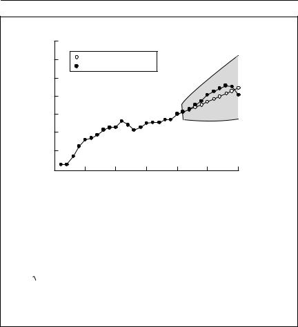
Forecasted population |
|
|
|
|
||
|
Actual population |
|
|
|
|
|||
|
|
|
|
|
|
|||
|
8 |
|
|
|
|
|
|
|
ln(deer) |
7 |
|
|
|
|
|
|
|
6 |
|
|
|
|
|
|
|
|
|
5 |
|
|
|
|
|
|
|
|
4 |
|
|
|
|
|
|
|
|
3 |
|
|
|
|
|
|
|
|
1910 |
1915 |
1920 |
1925 |
1930 |
1935 |
1940 |
|
|
|
|
|
Year |
|
|
|
|
To see how well the method of Dennis et al. (1991) forecasts population size, I derived r from the first 19 years of data, and then used it to predict N(t) for the next 10 years. Defining s as the number of years forward the forecast is required for, and n as the number of years from which the estimate of r is obtained, the standard error of N(s) is
seN(t) = & 2 s(1 + s/n).
The forecast value of N(t) is shown in the second figure, together with the observed N(t) and a 95% confidence interval. As the observed data keep within the confidence band, the projection is satisfactory up to 1940.
Allometric approaches
It is obvious that rmax is higher for bacteria than mice, and that in turn rmax is greater in mice than elephants. This allometric relationship between body size and the intrinsic rate of increase appears first to have been formally described by Smith (1954) and has since been investigated by a number of authors. The relationship has the potential to be used for estimating r in cases where reliable life-history or time-series data are unavailable.
Table 5.2 shows details of some of the allometric relationships reported in the literature, standardized to units of grams and days. There is no doubt that there is a highly significant relationship between log(rmax) and log(mass) both between taxa and within taxa, and that the relationship is close to linear. On theoretical grounds, the slope of the relationship can be predicted to be close to − 0.25 (Peters, 1983). In most cases, the estimated slope is remarkably
152 C H A P T E R 5
Table 5.2 Allometric relationships between rmax (d−1) and mass (g). Standard errors (where available) are given in brackets after the parameter estimate
Taxon |
|
Intercept |
|
Slope |
|
|
Sample size |
Source |
‘Unicellular organisms’ |
|
−1.936 7 |
|
− 0.28 |
|
|
26 |
Fenchel (1974) |
Heterothermic metazoa |
|
−1.693 1 |
|
0.273 |
8 |
|
11 |
Fenchel (1974) |
Homoiothermic metazoa |
−1.4 |
|
− 0.275 |
|
|
5 |
Fenchel (1974) |
|
Viruses to mammals |
|
−1.6 |
|
− 0.26 (0.012 6) |
|
49? |
Blueweiss et al. (1978) |
|
Mammals |
|
−1.872 1 |
|
− 0.262 |
2 |
|
44 |
Hennemann (1983) |
Mammals |
|
−1.31 |
|
− 0.36 |
|
|
9 |
Caughley and Krebs (1983) |
Mammals |
|
−1.436 0 (0.085 6) |
|
− 0.362 |
0 (0.026 6) |
84 |
Thompson (1987) |
|
Insects |
|
−1.736 0 (0.075) |
|
− 0.267 (0.097) |
|
35 |
Gaston (1988) |
|
|
–1 |
|
|
|
|
|
|
|
day) |
–2 |
|
|
|
|
|
|
|
) (per |
|
|
|
|
|
|
|
|
|
|
|
|
|
|
|
|
|
max |
|
|
|
|
|
|
|
|
r |
|
|
|
|
|
|
|
|
Log( |
–3 |
|
|
|
|
|
|
|
|
|
|
|
|
|
|
|
|
|
–4 |
1 |
2 |
|
3 |
4 |
5 |
|
|
0 |
|
|
|||||
Log(mass) (g)
Fig. 5.2 Regression of log10(rmax) versus log10(mass) using data from Thompson (1987). The dashed lines are 95% prediction intervals for estimation of log(rmax) for an individual species given its mass.
close to this value, the exceptions being the relationship derived by Caughley and Krebs (1983) (based on nine data points only) and Thompson (1987). Thompson’s method of calculation could be expected to overestimate the slope, as he used the equation of Cole (1954) (eqn (5.10)) to estimate r. Because this equation omits mortality before last breeding, it will overestimate r in all cases, but could be expected to do so particularly for mammals with small body sizes which have high juvenile mortality compared to larger mammals. Somewhat surprisingly, Hennemann (1983) estimates a slope in accordance with other studies, despite also using Cole’s method.
Despite the strength of these allometric relationships, they do not allow for accurate estimation of r. For example, Figure 5.2 shows the largest data set, that of Thompson (1987), together with a 95% confidence interval for the predicted r. At any mass, the interval spans almost an order of magnitude, an error that will make substantial differences even to the qualitative results of

R A T E O F I N C R E A S E O F A P O P U L A T I O N 153
most models. Allometric relationships should therefore be used as methods of last resort for predicting r, and only when life-history information is totally unavailable.
The ratio of production to biomass, P/B, is closely related to rmax. Paloheimo (1988) shows that, in an increasing population, P/B is equal to the sum of the rate of increase (in terms of biomass) and the biomass-weighted average mortality rate. In cases where population size is better described by biomass than numbers (for example, fisheries models) P/B is a more appropriate parameter to describe the potential rate of population increase. Allometric relationships between mass and P/B have been investigated by several authors (Banse & Mosher, 1980; Paloheimo, 1988; Boudreau & Dickie, 1989), particularly in marine organisms. In general, patterns are similar to those reported
for rmax.
Two features of the relationships are worth commenting on. First, there is apparently a stronger relationship between mass and P/B within taxonomic groups of marine organisms than there is overall (Boudreau & Dickie, 1989). Gaston (1988) reported the opposite pattern for rmax in insects, but this may be because insects within taxonomic groups covered relatively smaller size ranges. Second, somewhat surprizingly, P/B does not appear to depend on temperature (Banse & Mosher, 1980), at least over the range 5 –20˚C. This pattern was also reported by Gaston (1988). There appears to be little prospect of improving predictions of rmax or P/B by inclusion of ambient temperature in a regression.
Stochasticity
If an estimate of r is required for a stochastic model, a point estimate (a single value) for the rate of increase is not sufficient. It is necessary to quantify the variability of the rate of increase through time. This has been touched upon previously in the chapter, but it is important to understand that the standard error of r (eqn (5.18)) describes the accuracy with which the point estimate of r is known, and does not in itself quantify the variation in r through time.
The stochastic version of eqn (5.1) is
dN(t) = rN(t)dt + σN(t)dW(t). |
(5.19) |
Loosely, σ is the standard deviation of the variation in r and dW(t) is white noise, or uncorrelated random variation. This equation and its properties have been studied in considerable detail (Tuljapurkar, 1989; Dennis et al., 1991).
For practical purposes, however, it is much more common to use a discretized version of eqn (5.19),
N(t + 1) = N(t) + rN(t) |
(5.20) |
154 C H A P T E R 5
increaseof |
+0.5 |
|
|
|
|
|
|
|
|
|
|
|
|
|
|
|
|
|
|
|
|
|
|
|
|
|
|
|
|
|
|
|
|
|
|
|
|
|
|
|
|
|
|
|
|
|
|
||
|
|
|
|
|
|
|
|
|
|
|
|
|
|
|
|
|
|
|
|
|
|
|
|
|
|
|
|
|
|
|
|
|
|
|
|
|
|
|
|
|
|
|
|
|
|
|
|
|
|
rate |
0 |
|
|
|
|
|
|
|
|
|
|
|
|
|
|
|
|
|
|
|
|
|
|
|
|
|
|
|
|
|
|
|
|
|
|
|
|
|
|
|
|
|
|
|
|
|
|
||
|
|
|
|
|
|
|
|
|
|
|
|
|
|
|
|
|
|
|
|
|
|
|
||
|
|
|
|
|
|
|
|
|
|
|
|
|
|
|
|
|
|
|
|
|
|
|
||
|
|
|
|
|
|
|
|
|
|
|
|
|
|
|
|
|
|
|
|
|
|
|
||
|
|
|
|
|
|
|
|
|
|
|
|
|
|
|
|
|
|
|
|
|
|
|
|
|
|
|
|
|
|
|
|
|
|
|
|
|
|
|
|
|
|
|
|
|
|
|
|
|
|
|
|
|
|
|
|
|
|
|
|
|
|
|
|
|
|
|
|
|
|
|
|
|
|
|
Exponential |
–0.5 |
|
|
|
|
|
|
|
|
|
|
|
|
|
|
|
|
|
|
|
|
|
|
|
|
|
|
|
|
|
|
|
|
|
|
|
|
|
|
|
|
|
|
|
|
|
|
||
|
|
|
|
|
|
|
|
|
|
|
|
|
|
|
|
|
|
|
|
|
|
|
||
|
|
|
|
|
|
|
|
|
|
|
|
|
|
|
|
|
||||||||
|
–1.0 |
|
|
|
|
|
|
|
|
|
|
|
|
|||||||||||
|
|
|
|
|
|
|
|
|
|
|
|
|
|
|
|
|
|
|
|
|
|
|
|
|
0 |
200 |
400 |
600 |
800 |
0 |
200 |
400 |
600 |
800 |
|
Annual rainfall (mm) |
|
|
Annual rainfall (mm) |
|
||||
(a) |
|
|
|
|
(b) |
|
|
|
|
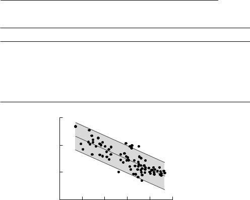
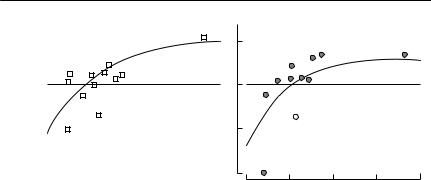
Fig. 5.3 The relationship between r and rainfall (lagged six months) for kangaroos. The figure shows this relationship for (a) red kangaroos, Macropus rufus, and (b) western grey
kangaroos, M. fuliginosus, on Kinchega National Park, western New South Wales. The fitted curves are r = − 0.57 + 1.14(1 − e−0.004R) (red kangaroos) and r = − 0.69 + 1.04(1 − e−0.005R)
(western grey kangaroos), where R is the annual rainfall. The relationship was calculated with a six-month lag: the annual rainfall in a calendar year was regressed against the rate of increase from 1 July of that year to 1 July of the next year. The open symbols were not used in calculating the fitted curves. From Bayliss (1987).
(see, for example Burgman et al., 1993). This can be iterated repeatedly over the time period of interest, sampling from a probability distribution for r, and the resulting frequency distributions for N(t) can be studied. The task is thus to find an appropriate probability distribution for r.
The most direct way this can be done is essentially identical to that described earlier. Given a time series of population sizes one time unit apart, the variance of r is estimated by the sample variance of ln(Nt/Nt−1). The difficulty with this approach is that it requires a long time series to derive a good estimate, and that the variance is simply one parameter of the probability distribution of r. It would usually be assumed that the distribution was approximately normal (Burgman et al., 1993).
A more indirect approach is to estimate the relationship between r and an environmental variable for which a long time series is available. This relationship can then be used to generate a probability distribution for r by sampling from the distribution of the environmental variable. In many terrestrial environments, rainfall is the obvious variable to choose. Even in a recently settled country like Australia, yearly records going back at least a century are available in most areas. For kangaroos, there is a very good relationship between rainfall and r (Bayliss, 1987; Cairns, 1989) (see Fig. 5.3). This has been used to generate the stochastic driving parameter in models of red kangaroos (Caughley, 1987) and adapted to generate stochastic variation in a model of bridled nailtail wallaby populations (McCallum, 1995a).

R A T E O F I N C R E A S E O F A P O P U L A T I O N 155
Why estimate r ?
Models requiring an estimate of r are usually general and at a high level of abstraction. They are typically ‘strategic’ rather than ‘tactical’ models, intended to provide a simple and general representation of a range of ecological situations, rather than a precise representation of any particular situation. As the model will only approximately represent the ecological processes operating, there is no point in putting large amounts of effort into rigorous statistical estimation of the parameter. A far more important problem is to ensure that the value of r being estimated is appropriate for the problem being examined.
For example, an important issue in bioeconomics is whether it is in the economic interests of a sole owner of a population to conserve it, or whether there is more economic benefit in elimination of the population and investment of the profits elsewhere. Clark (1973a; 1973b) has shown that extinction of a population is optimal if
1 + i > (1 + r)2 |
(5.21) |
and |
|
p > g(0), |
(5.22) |
where i is the discount rate (the yearly rate at which financial managers discount future versus current profits), p is the unit price of the animals, and g(0) is the cost of harvesting the last individual.
Clark’s analysis was based on a simple logistic model of population growth without harvesting, with equally simple economic elements. The dynamics of the harvested population are represented as
dN |
|
|
N |
|
|
|
|
= rN 1 |
− |
|
|
− EqN, |
(5.23) |
dt |
|
|||||
|
|
K |
|
|
||
where N is the size of the harvested population, K is the carrying capacity in the absence of harvesting, E is the harvesting effort and q is the catchability. The analysis was directed at baleen whale harvesting, but the same model has more recently been applied to elephant hunting (Caughley, 1993) and kangaroo harvesting (McCallum, 1995b).
Inspection of eqn (5.23) shows that r is being used to encompass all aspects of the population dynamics of the population other than resource limitation and harvesting. It is the long-term average rate of increase the population could sustain without resource limitation, not the rate of increase that could be sustained in unusually favourable environmental conditions.
There is limited value in estimating r for its own sake. The rate of increase usually is the output from a model, and there is little point in using it to forecast population growth using eqn (5.2). Almost always, the original ageor

156 C H A P T E R 5
stage-structured model will do a better job of projection than will plugging the estimate of r the model provides into eqn (5.2). This presupposes that the ageor stage-class composition of the population is obtained at the same time as the stage-specific mortality and fertility rates.
Summary and recommendations
1 The most appropriate definition and estimate of the rate of increase r is dependent on the context in which it is to be used. In many contexts, r is intended to represent the per capita growth rate of the population in the absence of all the other factors that are included in the model explicitly.
2 It is important to distinguish between: W, the observed rate of increase of a population; rs, the rate at which it would grow, given the current mortality and fecundity schedules, once a stable age distribution is reached; and rmax, the maximum rate at which a population of a given species could grow, in a given environment, without density-dependent constraints.
3 Given estimates of age-specific fecundity and age-specific mortality, rs can be estimated using the Euler–Lotka equation. Care needs to be taken in defining the fecundity terms correctly.
4 In the short term, a population may grow much faster than the rate rs predicted from its age-specific fecundity and mortality schedules.
5 The observed rate of increase of a population, W, can be estimated from time-series data. The most appropriate way to estimate this rate depends on whether the error in the time series is predominantly observation error or process error. If both are important, no currently available method is entirely satisfactory. Chapter 11 provides some suggestions on how to proceed.
6 Observation error occurs because the recorded values of population size are only estimates, and not the true population size. If observation error predominates, r can be estimated simply from the slope of a linear regression of ln(N) versus time (N is the estimated population size at time t).
7 Process error is variation in the actual size of the population, at a given time, from the size predicted by the model being used. If process error predominates, then r should be estimated from the mean of the change in ln(N ) between censuses one time unit apart.
8 There is a strong allometric relationship between the size of an animal and rmax. However, estimating rmax from adult body size should be considered only as a method of last resort.
9 If a probability distribution of r is required, a useful approach is to find a relationship between r and an environmental variable such as rainfall.