


Acknowledgements
I am very grateful to Tony Pople (University of Queensland) for reading several of the chapters, providing unpublished data, and performing some of the example calculations. I wrote part of the book whilst on Study Leave. I thank Ilkka Hanski (University of Helsinki), Bryan Grenfell (University of Cambridge) and Roy Anderson (Oxford University) for their hospitality, and for the productive discussions with them and their research groups. Support from the Australian Research Council also contributed to the book. Finally, I am very grateful for the patience of Blackwell Science, and the series editors, John Lawton and Gene Likens, throughout the gestation of this book.
I would also like to thank the following publishers and journals for allowing material from their publications to be used in this book: Academic Press: Fig. 10.9e (McCallum & Scott, 1994); Biometrics: Box 3.2 (Smith et al., 1995); Blackwell Science: Fig. 7.7 (van den Bosch et al., 1992); Canadian Journal of Fisheries and Aquatic Sciences: Fig. 6.2 (Walters & Ludwig, 1981), Table 6.3 (Getz & Swartzman, 1981); Chapman and Hall: Fig. 6.1 (Hilborn & Walters, 1992); Cambridge University Press: Fig. 5.3 (Bayliss, 1987), Box 9.1 (Peters, 1983); Ecology: Box 6.2 (Turchin & Taylor, 1992), Fig. 7.2 (Okubo & Levin, 1989), Fig. 8.5 and Table 8.2 (Pascual & Kareiva, 1996), Fig. 9.3c (Messier, 1994), Fig. 9.3d (Crawford & Jennings, 1989), Figs 9.8 and 9.9 (Carpenter et al., 1994), Fig. 10.10 (Dobson & Meagher, 1996); Epidemiology and Infection: Fig. 10.4 (Hone et al., 1992); Journal of Animal Ecology: Figs 10.7 and 10.8 (Hudson et al., 1992); Journal of Parasitology: Fig. 10.1 (Hudson & Dobson, 1997); Limnology and Oceanography: Fig. 4.4 (Hairston & Twombly, 1985); MacMillan: Fig. 2.1 (Swartzman & Kaluzny, 1987); Oecologia: Fig. 9.3b (Pech et al., 1992); Oikos: Figs 8.1 and 8.2 (Abramsky et al., 1992, 1994), Fig. 8.3 (Abramsky et al., 1994), Fig. 8.4 (Chase, 1996), Fig. 9.3a (Sinclair et al., 1990), Figs 9.4 and 9.5 (Caughley & Gunn, 1993); Oxford University Press: Fig. 10.9a and b (Anderson & May, 1991); Parasitology: Fig. 10.2 (Woolhouse & Chandiwana, 1992), Fig. 10.3 (McCallum, 1982), Fig. 10.6 (Gulland & Fox, 1992), Fig. 10.9c and d (Gulland, 1992); Princeton University Press: Figs 8.6 and 8.7 (Tilman, 1982 © 1982, reprinted by permission of Princeton University Press); Science: Fig. 6.3 (reprinted with permission from Myers et al., 1995 © 1995 American Association for the Advancement of Science), Box 7.1 (reprinted with permission from Wahlberg et al., 1996 © 1996 American Association for the Advancement of Science); Science of the Total Environment: Fig. 10.5 (Grenfell et al., 1992 © 1992, reprinted with permission from Elsevier Science); Trends
ix

xA C K N O W L E D G E M E N T S
in Ecology and Evolution: Figs 7.3 and 7.4 (Koenig et al., 1996 © 1996, reprinted with permission from Elsevier Science), Fig. 7.6a (Waser & Strobeck, 1998 © 1998, reprinted with permission from Elsevier Science); University of Chicago Press: Table 8.1 (Pfister, 1995), Figs 9.6 and 9.7 (Turchin & Hanski, 1997); Wildlife Monographs: Fig. 3.5 (Pollock et al., 1990).

C H A P T E R 1
Introduction
Scope of modelling
Any attempt to draw generalizations in science involves a model: an abstracted version of reality. A standard dictionary definition of a model is:
A simplified description of a system, process, etc., put forward as a basis for theoretical or empirical understanding.
(New Shorter Oxford English Dictionary)
This is a fairly accurate summary of the objective of ecological modelling. Models may be verbal or diagrammatic, but this book is concerned with
mathematical models: the subset of ecological models that uses mathematical representation of ecological processes. All statistical methods implicitly involve mathematical models, which are necessary in order to produce parameter estimates from the raw data used as input. This book is particularly concerned with models that use parameter estimates as input, rather than those that produce them as output. Statistical models are included only to the extent that is necessary to understand the properties and limitations of the parameter estimates they generate.
Scope of this book
This book concentrates on parameter estimation for models in animal population ecology. It does not attempt to deal with models in plant biology, nor to cover processes at the community or ecosystem level in any detail. I have biased the contents somewhat towards ‘wildlife’ ecology. The term ‘wildlife’ is a rubbery one, but it usually means vertebrates, other than fish.
I have not aimed to provide a full coverage of the methods required for parameter estimation in fisheries biology. Some fisheries-based approaches are included, largely where they have relevance to other taxa. As the branch of population ecology with the longest history of the practical application of mathematical modelling (although not with unqualified success: Beddington & Basson, 1994; Hutchings & Myers, 1994), fisheries has much to offer other areas of ecology. It has a large literature of its own, and to attempt a coverage that would be useful for fisheries managers, whilst also covering other areas of ecology, would be impractical. The classic reference on parameterizing fisheries models is Ricker (1975). An excellent, more recent treatment can be found in Hilborn and Walters (1992).
1

2C H A P T E R 1
I have written the book with two principal audiences in mind. First, wildlife managers in most countries are now required by legislation to ensure that populations, communities and ecosystems are managed on an ecologically sustainable basis. Any attempt to ensure sustainability entails predicting the state of the system into the future. Prediction of any sort requires models. Frequently, managers use packaged population viability analysis models (Boyce, 1992) in an attempt to predict the future viability of populations. These models require a rather bewildering number of parameter estimates. This book provides managers with clear recommendations on how to estimate parameters, and how to ensure that the parameters included in the model are the appropriate ones to answer particular management questions. Most population viability analysis models currently model a single species at a time. Parameters for single species are the topic of the first few chapters in the book. However, it is very clear that management decisions will increasingly require interactions between species to be taken into account. The final chapters deal with estimating parameters that describe interactions.
My second target audience is researchers in ecology, including postgraduate students. In addition to recipes and recommendations for parameter estimation in straightforward cases, I have reviewed some of the approaches that have been taken recently in specific, more complicated circumstances. These provide jumping-off points from which researchers can develop novel approaches for their own particular problems. For this audience, it was not possible to make the book entirely self-contained, but I hope it provides a good summary and entry into the current literature.
Almost the entire book is accessible to anyone who has completed an introductory ecology course, together with a biometrics course covering analysis of variance and regression. No computing skills beyond a familiarity with simple spreadsheets are assumed. Spreadsheets are an excellent tool for simple modelling and analysis, and are particularly good for working through examples to make ‘black boxes’ more transparent. I have used them extensively throughout the book. Beyond what can be done easily with a spreadsheet, there is little point in providing computer code or detailed instructions for applying particular numerical methods. There is now an enormous range of software available, both for general statistical analysis and for particular ecological estimation problems. Much of this software, particularly for specific ecological problems, is freely available on the World Wide Web. As the web addresses for software tend to move around, the Blackwell Science Web site (www. blackwellscience.com) should be consulted for current links.
Why model?
Before commencing any modelling exercise, it is absolutely essential to decide

I N T R O D U C T I O N 3
what the model is for. There is little point in constructing an ecological model if it is simply going to be placed on a shelf and admired, like a ship in a bottle. A model can be thought of as a logical proposition (Starfield, 1997). Given a set of assumptions (and these assumptions include estimates of the parameters used in the model), then certain consequences, or model outputs, follow. In this sense, all models make predictions. However, it has often been suggested that a distinction can be made between models developed for explanation and models developed for prediction (Holling, 1966; May, 1974b). Models for explanation are developed to better understand ecological processes. Their goal is to make qualitative predictions about how particular processes influence the behaviour of ecological systems. This means that they will usually be highly abstract and very general. As a result, they are likely to be quite poor at making accurate quantitative predictions about the outcome of any specific interaction. General models developed for understanding are often called ‘strategic’ models. A classic example of a strategic model is the model developed by May (1974a) to investigate the influence of time delays and overcompensation in populations with non-overlapping generations. This model has only one parameter, but it operates at such a high level of abstraction that there is little point in trying to estimate this parameter for any real population. To even begin to see which of the general properties of the model apply to real populations, it is necessary to use slightly more complex and realistic models (Hassell et al., 1976).
In contrast, ‘tactical’ models may be developed in an attempt to forecast quantitatively the state of particular ecological systems in specific circumstances. This is usually what is meant by a ‘predictive’ model. Such models must typically be quite complex and will often require a large amount of ecological data to generate estimates of a considerable number of parameters. The highly specific and complex models developed for the northern spotted owl (Lande 1988; Lamberson et al., 1992; Lahaye et al., 1994), are examples of tactical models. For such models to be valuable, it is absolutely essential that parameter estimates should be as accurate as is possible. For reasons I discuss at the beginning of the next chapter, do not assume that a complex model with many parameters will necessarily produce more accurate quantitative predictions than a simpler model.
These two examples represent ends of a continuum; in between are strategic models intended to provide general predictions about particular classes of ecological interactions, and tactical models intended to provide approximate predictions in the absence of detailed ecological data. Locating a model along this continuum is very important from the point of view of parameterizing models. There is little value in attempting to derive highly accurate parameter estimates for a strategic model. As they operate on a high level of abstraction, many processes are frequently subsumed into one parameter, making the

4C H A P T E R 1
translation from real biological data into an appropriate parameter estimate quite difficult. Parameter estimates for models of this type are also contextdependent. An estimate of the intrinsic rate of increase r for a particular species in a particular place that is appropriate for one abstract model may well be quite inappropriate for another model of the same species, in the same place, if that model has a different purpose (see Chapter 5). For a strategic model, estimates of the appropriate order of magnitude are typically required, and the principal problem is to ensure that the translation from biological complexity to mathematical simplicity is carried out correctly. One major advantage of simple models is that at least some results can be expressed algebraically in terms of the parameters. This means that the dependence of the results on particular parameters or combinations of parameters is obvious.
Models for prediction will usually require estimates of more parameters than models for understanding, and these estimates usually must be more accurate if the model is to be useful. Stochastic models require information on the probability distribution of parameters: the variance, shape of the distribution and correlation between parameters.
It is very tempting to be prescriptive, and demand that all parameter estimates should be based on sound experimental designs and rigorous statistical methods. Indeed, it is highly desirable that they should be, and the more rigour that can be introduced at the parameter estimation stage, the more reliable will be the results of the resulting models, provided the model itself is appropriate. However, rigour is a luxury that may not be affordable in many practical contexts. All management decisions in ecology are based on models, even if those models are verbal or even less distinct ‘gut feeling’. If it is decided not to use a mathematical model because the parameters cannot properly be estimated, the management decision will proceed regardless. We often are not able to postpone decisions until the appropriate experiments can be done. By that time, the species in question may have ceased to exist, or the ecosystem may have become irreversibly degraded.
It will usually be the case that a set of approximate parameter estimates in a formal mathematical model is preferable to an arm-waving argument. At least, in the former case, the assumptions on which the model is based will be transparent, and there is the possibility of investigating the robustness of the conclusions to the uncertainty in parameters and assumptions. Problems occur when the results of such modelling are presented to managers as coming from a black box, and no commitment is made to testing the assumptions and tightening parameter estimates so that the next version of the model is more reliable. It is also important to perform ‘sensitivity analysis’: to consider the range of model behaviour produced by the range of plausible values for the input parameters.
Successful applications of modelling in ecology are almost always iterative.

I N T R O D U C T I O N 5
The initial versions of the model highlight areas of uncertainty and weakness, which can then be addressed in later versions.
Brief taxonomy of ecological models
Continuous and discrete time
One of the major distinctions between models is whether they deal with time continuously or in discrete steps. Continuous-time models are usually structured as one or more differential equations, in which the rate of change of one or more variables (usually population size) is represented as a function of the various parameters and variables. The simplest of these is the equation for exponential growth
dN |
= rN , |
(1.1) |
|
||
dt |
|
|
which states simply that the rate at which the size of the population N increases with time is a constant r (the intrinsic rate of increase) times the current population size. This equation thus has a single parameter r to be estimated, but as will be seen in Chapter 5, this is not a straightforward task.
The principal advantage of differential equation models is that considerable progress can be made in understanding their behaviour analytically, using the standard tools of calculus. For an ecologist, the advantage of this is that the sensitivity of the model’s behaviour to changes in parameter values can be understood by looking at the algebraic structure of the analytic results, without the need for exhaustive and necessarily incomplete numerical sensitivity analysis. This process will be illustrated with an example in the next chapter. Only rarely, however, is it possible to obtain an algebraic closed form for population size as a function of time. That is, it is usually impossible to represent population size as
N(t) = f (t,p), |
(1.2) |
where N(t) is population size at time t, p is a set of parameters and f is an arbitrary function. Usually, it will be necessary to use a numerical algorithm to obtain an approximate result. All algorithms proceed by approximating the continuous process by a series of discrete steps. However, in contrast to discrete-time models, the step length is determined by the accuracy required, not the structure of the model itself; it can be made as small as necessary, and, using many algorithms, it can be altered as the solution is calculated. A good indication that the step length in a numerical solution of a continuous-time model is sufficiently short is if the solution does not change, depending on the step length.

6C H A P T E R 1
Discrete-time models, in contrast, represent time in fixed steps, the length of which is determined by the structure of the model itself. The simplest such models represent time in generations, and were first developed for univoltine insects: insects that have one generation per year, and in which offspring are not in the adult stage at the same time as their parents. Most genetic models also represent time in discrete generations (see, for example, Hartl & Clark, 1997).
The second major class of models that represent time in discrete steps are those developed for long-lived vertebrate populations (Caughley, 1977a). In these, the time scale is conventionally one year, and whilst generations will clearly overlap in a long-lived animal, the assumption is made that events occur sufficiently slowly that a good representation of population dynamics can be obtained by taking a ‘snapshot’ once a year. Such models will usually also include age structure.
Age and stage structure
Unstructured models represent the population size (or possibly biomass) of a given species with a single variable, aggregating all age classes and developmental stages together. This is quite appropriate for univoltine species if a snapshot of population size once per generation is adequate, and is sufficient for many abstract strategic models. The obvious advantage is that the model can be kept relatively simple, and the number of parameters required can be kept down.
In many cases, however, age or stage structure cannot be ignored. Different ages or stages may have very different reproductive rates, survival rates etc. Omission of such detail will make quantitative predictions quite inaccurate. Furthermore, there are considerable problems in attempting to derive appropriate aggregated parameters to use in unstructured models, if the input data are in either ageor stage-structured form. These problems and possible work-arounds are discussed in Chapters 4 and 5. Finally, the qualitative behaviour of structured models may be quite different from their unstructured equivalents. (For example, an invulnerable age class may change the behaviour of host–parasitoid or predator–prey models (Murdoch et al., 1987), and age-structured disease models may have much simpler behaviour than their unstructured equivalents (Bolker & Grenfell, 1993).) Even for very general strategic models, it is therefore worth exploring structured models, usually in comparison with, or in addition to, their unstructured counterparts.
There are numerous ways in which age or stage structure can be included in models, and readers should refer to some of the excellent books or reviews on the subject for details (e.g. Gurney et al., 1983; Nisbet & Gurney, 1983; Caswell, 1989). This section will outline briefly the types of such models from
I N T R O D U C T I O N |
7 |
Time |
|
Maturation |
|
Stage |
|
Death |
|
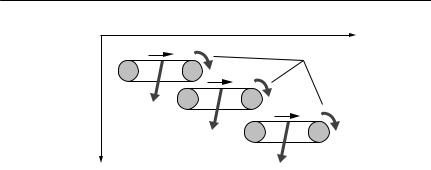
Fig. 1.1 The conveyor belt analogy for a structured population model. Each life-history stage can be imagined as a separate conveyor belt, which moves forward with time at a constant speed. The conveyor moves individual organisms through the life-history stage. They leave the stage either by falling off the belt (through death), or by reaching the end of the belt, at which point they mature into the next life-history stage. Organisms enter the first stage by birth, and the number of births is a function of the number of individuals
on one or more of the conveyors. All stages, other than the first, can be entered only by completing the previous stage. Death rates in a stage may be a function of population density of that stage, or other stages, and may vary with time. The length of each conveyor belt (the maturation time) may also vary dynamically according to environmental conditions or population density. This basic pattern underlies many structured population models discussed in the text, including the Leslie model (all conveyors are one time unit long), McKendrick–von Forster model (conveyors are infinitesimally short) and Gurney– Nisbett models. However, it cannot be used for some plant species (and only for a few animal species), in which differing modes of reproduction may cause individuals to enter different life-history stages, or in which regression from later to earlier stages is possible.
the point of view of parameter requirements. A good way to understand all such models is via a conveyor belt analogy, shown schematically in Fig. 1.1.
The Leslie matrix model (Leslie, 1945) is probably the best-known and most straightforward age-structured model. The population is divided into age classes of the same length as the time step (usually both are one year long). A proportion px individuals in age class x are then assumed to survive into the next age class, and the age-specific fertility (the number of female offspring in the first age class per female in age class x) is given by Fx. Methods to estimate these parameters, and some technical details of definition, are discussed in Chapter 4. Given these definitions, the vector of individuals in age classes 1 to n at time t + 1 can be derived from the numbers present at time t from the following matrix equation:
n1 |
|
F1 |
|
n |
|
p |
|
2 |
|
(t +1) = |
1 |
nx |
|
|
0 |
|
|
|
|
nk |
|
0 |
|
F2 |
Fx |
Fk |
n1 |
|
|
0 |
0 |
0 |
n |
|
(1.3) |
p2 |
0 |
0 |
2 |
(t). |
|
nx |
|
|
|||
0 pk−1 |
|
|
|
|
|
0 nk |
|
|
|||
This equation simply states that the only way to enter the first age class is by being born of a member of one of the age classes present at the previous
8C H A P T E R 1
time step, and that all subsequent age classes can only be entered by surviving through the previous age class in the previous time step. This simple model can generate only very simple behaviour: depending on the age-specific survivals and fertilities, the population will either grow or decline exponentially. Determining the rate at which it will do so is discussed in Chapter 5. The model is widely used in practice for short-term population projection, a task that can be accomplished very easily on a standard spreadsheet. A very full discussion of the Leslie model and others based on it is given by Caswell (1989).
The basic ideas of the Leslie matrix can be generalized fairly easily to cases in which stage classes are of differing lengths, so that individuals do not necessarily mature out of their current step in a given time step. Individuals can thus jump more than one step ahead, and even regress to a previous stage. Such models are often called Lefkowitz matrices. Again, Caswell (1989) has a full discussion of these models.
Simple matrix-based models can be very useful for practical purposes, particularly for short-term population extrapolation (see, for example, McDonald & Caswell, 1993; Heppell et al., 1994; Smith & Trout, 1994). They also form the basis around which more complex stochastic (random) models for population viability analysis are based (Burgman et al., 1993).
A further way of including age or stage structure in models has been developed by Nisbett and Gurney (Gurney et al., 1983; Nisbet & Gurney, 1983; Nisbet et al., 1989). This approach combines some of the analytic tractability of simple differential equation models with the realism of matrix-based models. In very general terms, time is treated as a continuous variable, so that there is no possibility that the model behaviour may be determined by the step length (as is the case with a matrix-based model). However, individuals cannot leave a life-history stage until a certain time period after entering it. Potentially, the maturation period may be a dynamic variable, determined by density-dependent processes or external variables. The principal disadvantage of the approach is that the model is formulated as a series of delay-differential equations. These are a little difficult to solve using either standard algorithms for the solution of differential equations or by elementary programming techniques.
McKendrick–von Forster equation
The most abstract age-structured model is the McKendrick–von Forster equation, which is a partial differential equation in which both time and age are continuous. Its derivation is not easy to explain. This version closely follows Caswell (1989). Define N(a,t) as the density of individuals of age a at time t. In other words, the number of individuals between the ages a1 and a2 at time t is given by

|
I N T R O D U C T I O N |
9 |
a=a2 |
|
|
|
N(a,t)da. |
(1.4) |
a=a1
This means that the number of individuals in the age interval (a,a + da) at time t is N(a,t)da. In the absence of mortality, after a short period dt all these individuals would be still alive, but dt older, so
N(a,t) = N(a + dt,t + dt).
Now, allow for mortality occurring at a per capita rate m(a,t), which may depend both on age and time. Then, the total number of animals of age a that die in the time period dt will be given by m(a,t)N(a,t)dt. Hence:
N(a,t) − N(a + dt,t + dt) = m(a,t)N(a,t). |
(1.5) |
This says simply that the difference between the number of animals that would be present if there was no mortality and the number that are actually present is the number that have died. All that it is necessary to do now is to note that
N(a + dt ,t + dt) ≈ N(a,t) + ∂N(a,t)dt + ∂N(a,t)dt.
∂ t ∂a
Substituting eqn (1.6) into eqn (1.5),
∂N ∂N
∂t + ∂a = −m(a,t)N(a,t).
(1.6)
(1.7)
Animals also are born, at which time their age is 0. The total rate of offspring production by individuals of age a at time t is given by the age-specific fecundity f(a,t) multiplied by N(a,t). Thus, the total number of animals of age 0 at time t is given by the boundary condition
∞ |
|
N(0,t) = f(a,t)N(a,t)da. |
(1.8) |
a=0
This model appears hard to understand. However, it is simply the result of taking the conveyor belt analogy in Fig. 1.1 to a limit in which each belt becomes infinitesimally short, but there is an infinite number of belts. The model is also difficult to parameterize. The task is one of choosing appropriate functional forms for both age-specific fecundity and mortality, both possibly as functions of time and other variables. Then all the parameters involved in these functional forms need to be estimated. Where the model has been used in practice, it has usually been approximated by one of the previous forms before parameter estimation was attempted. Nevertheless, the equation

10 C H A P T E R 1
is worth presenting as the general form of each of the more specific versions described above.
Deterministic and stochastic models
Deterministic models are those without a random component. This means that the population size in the next time period (or after an arbitrarily short time step in a continuous-time model) is entirely determined by the population size and structure at the current time, or, in the case of time-delayed models, by the previous history of population size and structure. In contrast, stochastic models include one or more random components, so that the population size in the future follows a probability distribution. It is a truism that the real world is stochastic, but nevertheless deterministic models are very valuable for some purposes.
The main advantage of deterministic models is their simplicity. As a rule, far more progress can be made in examining a deterministic model analytically than is possible with a stochastic model. Analytic results are always helpful, as it is much easier to deduce the influence of a particular parameter on a model’s behaviour if an algebraic representation of a result is available than if only a numerical result can be obtained. It is not necessary to solve a model fully, but algebraic representations of equilibria and their stability will provide very useful information. Even if only numerical solutions can be obtained, a single solution of a deterministic model represents its behaviour for a given set of parameters. In contrast, a single solution of a stochastic model may be quite unrepresentative of the ‘usual’ behaviour of the system for a particular parameter set. It is therefore essential to represent the probability distribution of outcomes at any particular time. Some approximations to the form of this distribution can sometimes be calculated analytically in simple cases (see Tuljapurkar, 1989), but usually it is necessary to calculate a large number of repeated solutions of a stochastic model for any set of parameters, and then to examine the frequency distribution of possible outcomes.
For some purposes, stochastic models are essential. Frequently, a problem may need to be approached with a combination of stochastic and deterministic models.
Deterministic models tend to be more suitable for strategic modelling, whereas tactical modelling is likely to require stochastic approaches. However, there are numerous examples of stochastic models being used for answering very general questions, and in many cases a simple deterministic projection model is sufficient to answer a specific problem about the likely future behaviour of a particular population. An excellent, but fairly technical discussion of stochastic modelling can be found in Tuljapurkar (1989). A much more accessible introduction to practical stochastic modelling is provided by Burgman et al. (1993).

I N T R O D U C T I O N 11
Using stochastic models introduces a series of problems additional to those of deterministic models. First, it is necessary to decide on what sort of stochasticity should be included. Second, it is necessary to determine appropriate forms for the probability distributions of the stochastic elements. Third, it is necessary to decide how the results should be presented. Stochasticity is often divided into three types, although these intergrade. Demographic stochasticity is randomness that occurs because the size of real populations can take only integer values. If an age class of 20 individuals has a probability of survival over a year of 0.5, this does not mean that exactly 10 individuals will survive, only that a random number sampled from a probability distribution with a mean or expected value of 10 will survive. If only demographic stochasticity is operating, the probability distribution of this random variable will be binomial. In addition to demographic stochasticity, there is randomness introduced because the environment is not constant. Environmental variation will cause the survival of 0.5 in the example above to change from year to year, although it may have a long-run mean of 0.5. There is no reason why environmental stochasticity should follow any particular probability distribution: it will depend on the nature of the environment, the parameter concerned, and the ecology of the organism in question. It is therefore much harder to make generalizations about the influence of environmental stochasticity on populations than it is for demographic stochasticity (see, for example, Goodman, 1987; or Lande, 1993). Ways in which appropriate probability distributions for environmental stochasticity in various parameters may be added to models are discussed in several chapters. Finally, many authors (e.g. Ewens et al., 1987; Lande, 1993) consider catastrophic stochasticity separately from environmental stochasticity. Catastrophic stochasticity is usually defined as the effect of random factors that may kill a large proportion of a population, irrespective of its size. It is really just an extreme form of environmental stochasticity, but appropriate ways to model it and its effects are often qualitatively different from most other forms of environmental variation.
All the above can be grouped together as process error. They are sources of random variation that cause the actual population to vary. In addition to process error, almost all ecological data will be subject to observation error. Observations of any quantity at all are unlikely to be the actual values, but instead are random numbers hopefully clustered around the actual value, with a sampling error. The distinction between process and observation error is important, as methods designed to operate in the presence of only one of these the sorts of error may be unreliable if the other source of error is dominant, or if both are important. This problem will be dealt within specific circumstances as it occurs.
For many ecological models, it is necessary not only to estimate the mean value of a parameter, but also to estimate some of the properties of its

12 C H A P T E R 1
frequency distribution. This is most obvious for stochastic models: if you wish to know the influence of a varying death rate on population size, it is self-evident that you need to know something of how that death rate varies through time. However, if any process is nonlinear (and most ecological processes are), then the behaviour of a deterministic model will be influenced by the frequency distribution of the parameters in the population and not just their mean values. For example, the most crucial parameter in most epidemiological models is R0, the reproductive number of the disease (Anderson & May, 1991). If R0 > 1, the disease will increase, but if R0 < 1, the disease will not persist. R0 cannot simply be estimated from the mean number of contacts per infected individual. It is necessary also to estimate the variance in the number of contacts, and the larger the variance for a given mean contact rate, the greater is R0 (Woolhouse et al., 1997). R0 and other parameters associated with host pathogen interactions are discussed in Chapter 10.
Together with the estimate of a given parameter, most standard statistical methods will return a standard error. This is an estimate of the precision with which the mean value of the parameter in the sampled population has been estimated, and it is thus a property of the sampling distribution. The sampling distribution may be related to, but is not the same as, the distribution of the parameter itself in the sampled population. In the simplest case, if a parameter has a normal distribution in a population, with a variance σ 2, the standard error of an estimate of the population mean from a sample of size n will be √(σ 2/n). However, if the parameter itself does not have a normal distribution, the problem is not as straightforward.
Individualand event-based models
Most stochastic models operate using a relatively small number of classes of individuals, and then use standard probability distributions (binomial, Poisson etc.) to generate the number of individuals in each class, at each successive time step. An alternative approach is to attempt to follow each individual in the population from its birth, through growth, dispersal and reproduction, to death (Rose et al., 1993; Judson 1994; Lomnicki, 1988). Such a model obviously requires more computer storage space and processing than one which deals with a small number of aggregated categories, but this is no longer the serious constraint it once was. Conceptually, such models are often quite simple, as only very elementary probability theory is necessary to construct them. The number of parameters and difficulties in estimation are frequently no greater than for an equivalent structured model, as individuals will usually be grouped into categories for parameterization purposes. Individual-based models hold particular promise for combining genetic and ecological processes, as even the most elementary genetic structure rapidly complicates the

I N T R O D U C T I O N 13
structure of any ecological model (see, for example, Beck, 1984; Andreasen & Christiansen, 1995).
Event-based models are a second form of calculation-intensive stochastic model. Rather than imposing a fixed time step on the model, they model each event (birth, death etc.) as it occurs. The approach was first suggested nearly 40 years ago (Bartlett, 1961), but has not often been used (but see Bolker & Grenfell, 1993). The basic idea is very straightforward. Suppose that there are three events, A, B and C, that could occur to a population at a given time t, and that they occur at rates a, b and c per unit of time. These rates can change through time, possibly depending on population size or any other internal or external variable. Then the waiting time to the next event has a negative exponential distribution with mean 1/(a + b + c). Which of the events occurs after this waiting time simply depends on the relative sizes of the rates: it will be A with a probability a/(a + b + c), B with a probability b/(a + b + c), etc. The negative exponential is a particularly easy distribution to generate on a computer (Press et al., 1994), and thus iteration is both straightforward and fairly quick. The event-based approach is probably the best way of numerically solving a continuous-time stochastic model, although if populations are large, individual demographic events may happen so rapidly that solution is very slow.