


C H A P T E R 7
Spatial parameters
Introduction
The importance of spatial processes in population dynamics has increasingly been recognized by ecologists in recent years (Levin, 1992). For some ecological questions, spatial dynamics are quite explicitly part of the problem. It is clearly nonsensical, for example, to attempt to predict the rate of spread of an invading species without a spatial component in the model. However, it has also become apparent recently that the qualitative behaviour of interspecific interactions (host–parasitoid, predator–prey and competitive) may be totally different in spatially heterogeneous environments than in the homogeneous environments implicitly assumed by most basic models (Hassell et al., 1991a; 1994).
Models may represent spatial processes at several levels of abstraction. Spatially explicit models (sometimes called landscape models) seek to represent populations, or even individuals, within the actual heterogeneous landscape that they inhabit (Dunning et al., 1995). Such models will usually represent the landscape as a series of cells that may be occupied by one or more individuals of the species under study, with the properties of the cells determined from a Geographic Information System (GIS). Movements and the various ecological processes acting on the occupants of the cells are then functions of the cell properties. Models of this type have been developed for the spotted owl (Strix occidentalis) in old growth forests of the western United States (Lamberson et al., 1992) and also for the endangered Bachman’s sparrow (Aimophila aestivalis) in the southeastern United States. Any such model will inevitably require large numbers of parameter estimates and it is unlikely that field data suitable for estimating all of these reliably will be available, even for the most well-known species (Conroy et al., 1995; Dunning et al., 1995).
Cellular automaton models (Caswell & Etter, 1993; Tilman et al., 1997) are a more abstract version of spatially explicit models. Again, the environment is divided into a large number of cells, and interactions are more likely to occur between close neighbours than cells far apart (in standard cellular automaton models, only neighbouring cells contribute to transition rules for each cell). The state of each cell is described by a binary variable (usually presence or absence). Cells are considered to be identical or of a relatively small number of types, so that despite the very large number of cells, the number of parameters needed is much smaller than in a spatially explicit model. The abstract nature
184

S P A T I A L P A R A M E T E R S 185
of these models means that they are valuable for exploring the qualitative influence of spatial structure on population dynamics, rather than for making accurate quantitative predictions about particular species in particular habitats.
Lattice models (e.g. Rhodes & Anderson, 1997) are a more complex version of a cellular automaton model. As with a cellular automaton model, interactions occur only (or primarily) between adjoining cells. In lattice models, however, each lattice point may contain more than one individual organism, and more than one interacting species.
Patch models incorporate a number of patches with particular properties and a specified spatial distribution, and then attempt to model dynamics within patches, together with the rate of movement between patches (for example, Lindenmayer & Lacy, 1995b). As with spatially explicit models, the number of parameters and thus the data requirements are substantial. More abstract versions of these models, with more modest numbers of parameters, include classical metapopulation models, in which only presence or absence on a patch is modelled, and patch models in which all patches are assumed to be equidistant.
Finally, reaction–diffusion models are based on models in physics that describe diffusion of heat across a surface or a solute through a liquid (Murray, 1989). Spatial spread is modelled in continuous space using partial differential equations. An excellent and succinct introduction to these models is provided by Tilman et al. (1997).
Corresponding to these levels of abstraction, spatial information will be needed with varying degrees of resolution. At the finest scale, the level of the individual organism, data may be required on home range, foraging range or territory or dispersal and migration distances and directions. At the level of the individual population, the numbers or proportions of individuals immigrating or emigrating per unit of time may be needed. At the level of the metapopulation, or group of populations, estimates of the extinction and colonization rates of each habitat patch or population may be required. At the highest level of abstraction, models operating in continuous space require estimates of the diffusion rate (or rate of spread through space) of the organisms.
Parameters for movement of individuals
Information on individual movements can be required in a model for several reasons. First, knowledge of home range or territory size will help determine the boundaries of the population under study. Is it appropriate to consider your population at the scale of square metres, hectares or square kilometres? Second, and more importantly, the range of an individual defines the environment in which it lives, in terms of resources, potential competitors and potential exploiters. In a spatially explicit model, the size of the home range

186 C H A P T E R 7
will determine either the size of the cells (if each cell represents a territory) or the number of cells each individual occupies. Similarly, dispersal and migration information are necessary to define the appropriate scale for modelling and the environment of the target organisms.
Collecting data
Almost all methods for collecting data about movements of individuals rely on capturing animals, marking them and then either following them, or recapturing or resighting them at some time or times in the future. It is beyond the scope of this book to describe methods for marking, tracking or relocating animals in any detail. Tracking methods vary in sophistication from following footprints in snow (Messier & Crête, 1985) or attaching reels of cotton to animals’ backs (Key & Woods, 1996) to radiotelemetry (see White & Garrott, 1990, for an excellent review), use of radioactive tracers (Stenseth & Lidicker, 1992) and satellite tracking (Grigg et al., 1995; Tchamba et al., 1995; Guinet et al., 1997). Do not assume that technologically sophisticated methods are necessarily the best. Given a constraint of fixed cost, there is always a trade-off between cost per sample and sample size.
Standard methods for survival analysis and population estimation based on mark–recapture or mark–resight are discussed in Chapter 4. If locations of initial capture and resight or recapture are recorded, then obviously some information on ranging behaviour is available. Equally obviously, a home range thus determined will usually be only a subset of the true range.
Analysis of range data
The home range of a species was originally defined as ‘that area traversed by an individual in its normal activities of food gathering, mating and caring for young’ (Burt, 1943). It is thus not necessarily a defended territory, and neither is it defined by the extreme bounds of the area within which the individual moves.
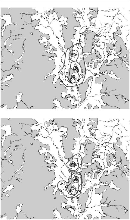
The simplest way of defining a home range is by a convex polygon, which is an envelope drawn around all available locations in such a way that all internal angles are less than 180˚ (see Fig. 7.1). As a means of defining the limits of the parts of the habitat used by an individual, a minimum convex polygon has several problems. First, it is determined by extreme observations, and will therefore be greatly affected by outliers. Second, it will be strongly influenced by sample size: the more points, the greater will be the minimum convex polygon. Third, if the habitat is patchy, the minimum convex polygon may include regions into which the animal never goes, if these areas are bounded by or surrounded by suitable habitat (White & Garrott, 1990).

S P A T I A L P A R A M E T E R S 187
Because of the limitations of the minimum convex polygon, various alternatives involving more sophisticated statistical analysis have been suggested. For example, Jennrich and Turner (1969) described a home range using a bivariate normal distribution. As this restricts the shape of the home range to an ellipse, its practical application is severely limited. More recent approaches have taken the approach of smoothing and interpolating the frequency distribution of locations, without imposing any particular shape upon them a priori. Two such approaches are the harmonic mean method (Dixon & Chapman, 1980) and kernel estimation methods (Seaman & Powell, 1996).
Migration and dispersal
A distinction is often drawn between dispersal, which is a spreading or movement of individuals away from others (diffusive movement), and migration, which is a mass movement of individuals from one place to another (advective movement) (Begon et al., 1996a, p. 173). However, the distinction cannot be applied too rigidly. Depending on the objectives of the model being constructed, the quantities that require estimation might include:
1 The probability distribution of distance moved by individuals, per unit of time. This might be considered either migration or dispersal, depending on whether movements were away from, or together with, conspecifics.
2 The probability distribution of the distance between the location of adults and the settlement point of their offspring, or equivalently, the probability distribution of the distance between the position of birth and the position of first reproduction. This would normally be considered to be dispersal.
3 For a given patch or subpopulation, the probability that an individual leaves it, per unit of time, or the number of individuals entering or leaving
Fig. 7.1 (on following pages) Home ranges for bridled nailtail wallabies (Onychogalea fraenata), as determined by various methods. These maps show an area in Idalia National Park, western Queensland, where a reintroduction of the endangered bridled nailtail wallaby is being attempted. The unshaded areas along drainage lines are potentially wallaby habitat, whereas the shaded areas are residual outcrops, unsuitable as habitat for these animals. The dots on each map are daytime sheltering locations obtained by radiotelemetry, over six months, for about 30 animals. The composite home ranges were calculated using the package CALHOME (Kie et al., 1996). For all but the convex polygon 50%, 75% and 95% utilization contours are plotted. From F. Veldman and A.R. Pople, University of Queensland (unpublished data). (a) Convex polygon. This encompasses all data points, but includes large amounts of habitat where animals were never found. (b) Jennrich–Turner bivariate normal distribution. This always will have an elliptical shape, whatever the actual pattern of space use. (c) Harmonic mean. This distribution is no longer constrained to have a particular shape, but substantial areas of unused habitat are still included. (d) Kernel estimator. This has done the best job of indicating where the animals actually were. The ‘square’ shape of some of the utilization contours is an artefact caused by the grid used to calculate the distribution.
188 C H A P T E R 7
0 |
1 |
2 |
3 |
4 |
5 |
km |
(a)
(b)
S P A T I A L P A R A M E T E R S 189
|
|
|
|
|
|
|
|
|
|
|
|
|
0 |
1 |
2 |
3 |
4 |
5 |
km |
||||||
(c)
(d)

190 C H A P T E R 7
it, per unit of time. These patch-specific entering and leaving processes are usually called emigration and immigration.
4 For a network of patches or subpopulations, the probability of movement, or the numbers of individuals moving, between each pair of patches. These rates are usually called migration rates. Typically, they may be functions of the physical size of each patch, any other measure of ‘quality’ of patches, population density in patches, and distance between, or arrangement of, patches in space.
The first two types of quantity are likely to be estimated from raw data consisting of distances moved by individuals, either animals that have been followed through time, or animals that have been marked at a particular location and subsequently recaptured, recovered, or resighted at another. For almost all distance-based movement data, it is essential to describe a probability distribution of distance moved. Almost always, the probability distribution of distance moved is highly skewed, so that the mean dispersal distance is a poor indication of the distance that ‘most’ individuals move. On the other hand, many important biological processes (such as the rate of spread of the population) are dependent on the tails of the distribution (how far a few animals manage to disperse) rather than on the mean (Kot et al., 1996).
Patch-related movement statistics, such as (3) and (4) above, are likely to be estimated from mark–recapture data, giving proportions of individuals marked on particular patches that are subsequently recovered on that patch, or on other patches. Genetic data are also increasingly being used to determine the extent to which subpopulations are isolated from each other.
Probability distributions of movement or dispersal distances
The probability distribution of dispersal distance is usually assumed to be negative exponential,
f (x) = ae−bx |
(7.1) |
where f(x) is the probability density of dispersal at distance x and a and b are constants; or sometimes is assumed to follow a power relationship,
f (x) = ax−b |
(7.2) |
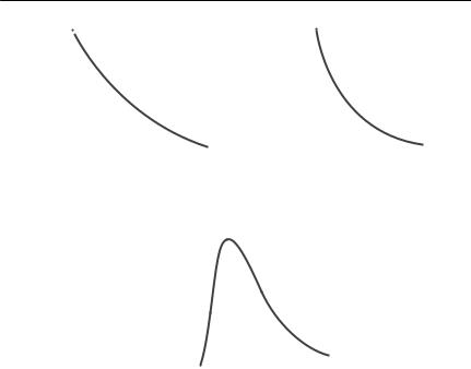
(Okubo & Levin, 1989). These relationships are phenomeological: that is, they are chosen because they seem to represent observed distributions of dispersal data quite well. Both distributions are monotonically decreasing, and will therefore fail to fit dispersal distributions which have a maximum at a distance greater than 0. Such distributions might be produced from the seed rain from tall trees (Okubo & Levin, 1989), or from larvae of marine species that have a fixed pre-patent period and are released into a net current flow. An example of the latter would be crown of thorns starfish larvae on the Great Barrier Reef
Probability density (y)
(a)
S P A T I A L P A R A M E T E R S 191
1.0 |
|
|
|
|
|
|
|
|
|
|
|
density (y) |
1.0 |
|
|
|
|
|
|
|
|
|
|
|
|
|
|
|
|
|
|
|
|
|
|
|
|
|
|
|
|
|
|
|
|
|
|
|
|||||
0.5 |
|
|
|
|
|
|
|
|
|
|
|
0.5 |
|
|
|
|
|
|
|
|
|
|
|
|
||
|
|
|
|
|
|
|
|
|
|
|
Probability |
|
|
|
|
|
|
|
|
|
|
|
|
|||
|
|
|
|
|
|
|
|
|
|
|
|
|
|
|
|
|
|
|
|
|
|
|
|
|
||
0.0 |
|
|
|
|
|
|
|
|
|
|
|
|
|
0.0 |
|
|
|
|
|
|
|
|
|
|
|
|
|
|
|
|
|
|
|
|
|
|
|
|
|
|
|
|
|
|
|
|
|
|
|
|
|||
0 |
1 |
2 |
3 |
|
4 |
5 |
|
|
0 |
1 |
2 |
3 |
4 |
5 |
||||||||||||
|
|
|
Distance (s) |
|
|
|
|
(b) |
|
|
|
|
|
Distance (s) |
|
|
|
|
||||||||
|
|
|
|
|
density (y) |
1.0 |
|
|
|
|
|
|
|
|
|
|
|
|
|
|
|
|
|
|
|
|
|
|
|
|
|
|
|
|
|
|
|
|
|
|
|
|
|
|
|
|
|
|
|
|
|||
|
|
|
|
|
0.5 |
|
|
|
|
|
|
|
|
|
|
|
|
|
|
|
|
|
|
|
||
|
|
|
|
|
Probability |
|
|
|
|
|
|
|
|
|
|
|
|
|
|
|
|
|
|
|
||
|
|
|
|
|
|
|
|
|
|
|
|
|
|
|
|
|
|
|
|
|
|
|
|
|||
|
|
|
|
|
|
|
|
|
|
|
|
|
|
|
|
|
|
|
|
|
|
|
|
|
||
|
|
|
|
|
|
|
0.0 |
|
|
|
|
|
|
|
|
|
|
|
|
|
|
|
|
|
|
|
|
|
|
|
|
|
|
|
|
|
|
|
|
|
|
|
|
|
|
|
|
|
|
|
|
|
|
|
|
|
|
|
|
|
|
0 |
1 |
2 |
3 |
|
4 |
|
5 |
|
|
|
|
|
|
|||||
(c) |
Distance (s) |
|
Fig. 7.2 Dispersal distributions: (a) negative exponential; (b) power; (c) Gaussian plume. In each case, the horizontal axis shows the distance from the source s, and the vertical axis is the probability density of settling propagules, y. From Okubo and Levin (1989).
(Scandol & James, 1992). Dispersal distributions of this type may be represented by Gaussian plume models (Okubo & Levin, 1989), which are based on a mechanistic representation of a plume of propagules that diffuses and is dispersed by wind or current. Figure 7.2 shows some theoretical dispersal distributions that can be generated by exponential, power and Gaussian plume models.
There are several ways in which data might be collected to determine a probability distribution for dispersal distance. Unfortunately, there are substantial biases associated with some methods. These biases are frequently not recognized (Koenig et al., 1996). One approach, developed most fully for dispersal of seeds or spores (Fitt & McCartney, 1986), is to use collectors of a given surface area at various distances from the source. This approach might also be applied to dispersal of invertebrates, or to any other situation where settlement of very large numbers of dispersers or propagules from a single source can be recorded. The number of individuals recovered per collector, as a function of distance, is not an estimate of the probability distribution of dispersal distance of individual propagules. The problem is that almost all

192 C H A P T E R 7
dispersal clouds expand as they disperse. The simplest model is that dispersal is uniformly distributed over a circle, or a segment of a circle. If this is the case, the area of settlement increases as the square of distance. The result is that the numbers of individuals settling per unit area would decline following an inverse square relationship, given a uniform probability distribution of dispersal distance.
Estimating the parameters a and b in eqn (7.1) or (7.2) for data of the above type is often done by log-transforming the cumulative proportion of individuals dispersing to particular distances, and then using conventional regression (e.g. Hill et al., 1996). This approach is technically incorrect, as cumulative proportions are not independent observations. This is the same problem as occurs with estimating survival rates by a regression of log survivors against time (see Chapter 4). The solution is also the same. The dispersal distance of each individual should be considered as an independent observation, with a negative exponential distribution. This means that a standard survival analysis program with a constant hazard rate can be used, substituting ‘distance’ for time (for eqn (7.1)) or log(distance) for time (for eqn (7.2)). Alternatively a generalized linear model with a gamma errors, a scale parameter of 1, and a reciprocal link can be used (see Crawley, 1993).
In cases where the modal dispersal distance is greater than zero, survival analysis approaches using a Weibull distribution (see Chapter 4) should be considered. They will not give results identical to the Gaussian plume models of Okubo and Levin (1989), but should produce qualitatively similar results.
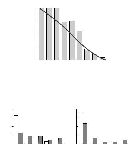
In many studies of vertebrate dispersal, an area of finite size is studied intensively. Within this area, individuals are marked, and their position at a later date is recorded. Only movements within the study area are recorded with high reliability, although there may be haphazard records from outside the main study area. Such a methodology will result in underestimates of the mean or median dispersal distance, unless dispersal distances are much smaller than the dimensions of the study area (Koenig et al., 1996). The problem is simply that dispersal events that take the animal beyond the study boundary are not recorded. The consequence is not just a truncation of the frequency distribution of dispersal. Because some individuals initially quite close to the study boundary will disperse out of the study with only a small movement, the effect is to generate a distribution of dispersal distances that appears to decline with distance, even if the true distribution is uniform (see Fig. 7.3). If there is no preferred direction of dispersal, the study area is circular, and individuals are distributed randomly throughout the area, Barrowclough (1978) provides a means of correcting for this type of bias. These are, however, restrictive assumptions that limit the validity of this correction.
Radiotelemetry generally will provide better estimates of the distribution of dispersal distances than will direct observation (Koenig et al., 1996), simply
|
|
|
S P A T I A L P A R A M E T E R S |
193 |
|
1.00 |
|
|
|
frequency |
0.75 |
|
|
|
0.50 |
|
|
|
|
Relative |
0.25 |
|
|
|
|
|
|
|
|
|
0.00 |
|
|
|
|
0 |
R |
D |
|
Dispersal distance
Fig. 7.3 The effect of a finite study area on observed dispersal distance. The frequency distribution of observed dispersal distances of 141 female acorn woodpeckers (Melanerpes formicivorus) within a finite study area is shown, overlaid with the probability of detection of a given dispersal distance, if dispersal directions are random and the study area is circular with radius R. Despite the apparent shape of the distribution, the observed distribution is quite consistent with a uniform distribution of dispersal distances over distances between
0 and D. From Koenig et al. (1996).
Individuals located (%)
(a)
100 |
|
|
|
|
100 |
|
|
|
|
75 |
|
|
|
|
75 |
|
|
|
|
50 |
|
|
|
|
50 |
|
|
|
|
25 |
|
|
|
|
25 |
|
|
|
|
0 |
<2 |
<3 |
<5 |
>5 |
0 |
<2 |
<3 |
<5 |
>5 |
<1 |
<1 |
||||||||
|
Distance (km) |
|
(b) |
Distance (km) |
|
||||
|
|
|
|
|
|
|
|
|
|
Fig. 7.4 Natal dispersal in yellow-bellied marmots (Marmota flaviventris): (a) Dispersal distances for males, based on intensive observation and trapping (unshaded bars) compared with those from radiotelemetry (shaded bars) (18 trapped, 52 radiotracked). (b) Dispersal distances for females, represented similarly to (a) (22 trapped, 38 radiotracked). From Koenig et al. (1996).
because fewer long dispersal distances will be missed. Figure 7.4 shows an example of natal dispersal distances in marmots that emphasizes this point.
Using mark–recapture methods to estimate migration rates
Applied to a single population, standard open-population methods for mark–recapture analysis (see Chapter 4) produce estimates of the number of new entrants to the population between sampling occasions. The methods

194 C H A P T E R 7
themselves cannot discriminate between offspring produced by the population under study and immigrants. In some cases, it will be obvious that the new entrants cannot be recently recruited juveniles. It will rarely be possible to distinguish between new recruits that have arisen from reproduction within the population and new recruits that have migrated into the population, but have arisen from reproduction outside it. These methods also estimate ‘survival’: the probability that individuals present in the population on one occasion are still present on the next trapping occasion. The methods cannot distinguish between death and permanent emigration. Temporary emigration, in which individuals leave the sampled population for one or more trapping occasions, but subsequently return, is a problem for mark–recapture methods. All such methods behave badly if the probability of capture varies substantially between individuals. If animals temporarily leave the population, then their probability of capture whilst they are absent is zero, and clearly this is different from the capture probability of those animals that remain in the population. Kendall et al. (1997) describe some possible ways of dealing with, and estimating the rate of, temporary emigration.
Tag–recovery studies, in which large numbers of animals are tagged, and recoveries of tagged animals are later reported, are commonplace in fisheries research and in ornithology. A major objective of such studies is to investigate movements, but the data are usually only analysed qualitatively. Typically, animals will be reported to have moved at least x kilometres, or y% of recoveries will be reported to have occurred within a certain distance of release. Information of this type is adequate to determine how far some animals can move, but not to quantify the amount of interchange between subpopulations, or to determine the frequency distribution of movements.
If animals are marked and recaptured or recovered from different subpopulations, it is possible to analyse recovery data more formally, to estimate the probability of movement between subpopulations or patches. The approach is an extension of standard mark–recapture methods for single populations. Instead of estimating φi, a single parameter representing the probability of survival from time period i to i + 1, the objective now is to estimate a matrix <i of survival/migration probabilities. Each element φirs in the matrix is the probability that an individual present in subpopulation r at capture occasion i is alive and present in subpopulation s at capture time i + 1. The diagonal elements of the matrix are thus simply the probabilities that animals are alive and have not moved from particular subpopulations, whereas the other elements are the probabilities that the animal has both survived and moved from subpopulation r to subpopulation s. It is impossible to separate migration probability from survival probability, without making certain restrictive assumptions (for example, that survival is identical in all subpopulations, or that movements only occur immediately before recapture).
Not surprisingly, the technical details of fitting these models are not straight-

S P A T I A L P A R A M E T E R S 195
forward. The basic approach is an elaboration of the standard Cormack–Jolly– Seber model (see Chapter 4). The raw data will consist of a series of capture histories, giving the stratum in which the animal was captured on each sampling occasion. For example, if there are three subpopulations A, B and C, and six capture occasions, the history 0AA0B0 would represent an animal first captured on the second sampling occasion in subpopulation A, recaptured the next time still in A, missed on the next occasion, picked up again in subpopulation B on the fifth occasion, and then not seen again. (In a mark–recovery study, as distinct from a mark–recapture study, there will only ever be one recapture.)
From these histories, the objective is to estimate the survival/migration parameters φirs (as defined above), and also the capture probabilities pis, (each pis is the probability of recapture at sampling time i for an animal present in subpopulation s at that time). As is the case with a standard Cormack–Jolly–Seber model, the estimates for the survival/migration parameters and capture probabilities over the last time interval are confounded: it is not possible to separate animals that were not captured, but were present, in a given subpopulation on the final sampling occasion from those that were no longer present.
For even a fairly small number of subpopulations, the number of parameters to be estimated rapidly becomes prohibitive. Brownie et al. (1993) suggest investigating reduced models, in which either or both the transition probabilities φ or the recapture probabilities p are considered to be constant through time, but variable across subpopulations. However, they also suggest that an additional complication may be necessary. The model, as described above, is ‘memoryless’ or Markovian. The probability of an animal moving from one population to the next depends only on where it currently is, not where it has been in the past. If some animals are ‘transients’ and others are ‘residents’, this will not be a reasonable assumption.
In addition to the standard parameters φ and p, some derived parameters based on these are likely to be of ecological interest, perhaps more than the original parameters themselves. For example,
s
φ r. = Σφrj (7.3)
j=1
is the total probability of survival through the time period (i,i + 1) of the animals present at time i in subpopulation r, wherever they end up, and
Ψrs = |
φ rs |
(7.4) |
|
φ r. |
|||
|
|
is the probability that an animal which was in subpopulation r at time i is present in subpopulation s at time i + 1, given that it has survived. If it can be assumed that movement occurs just before recapture, or that survival rates

196 C H A P T E R 7
within subpopulations are equal, eqns (7.3) and (7.4) enable survival and migration to be disentangled.
If independent data on population size in each subpopulation are available, the number of immigrants into or emigrants from each subpopulation can also be calculated (see Schwartz et al., 1993).
These methods are likely to be unreliable if animals make multiple moves and recapture rates are relatively low. For example, if the capture history
A 0 0 0 B 0
is recorded, it is not possible to determine whether the animal has survived in subpopulation A for three intervals, but has been missed, and has then migrated to B, or whether it has moved to B in the first time interval, but then has been missed whilst in B until capture occasion 5. It may even have gone to B, returned to A and then gone back to B, or even have gone to B via C. In most studies, migration is likely to be relatively unusual, so that multiple migration is rarer still.
The details of the calculations to estimate these parameters are in Brownie et al. (1993) (multiple recaptures) or Schwartz et al. (1993) (tag–recovery). Few ecologists are likely to want to undertake the calculations from scratch. The program MSSURVIV is available to estimate them (Hines, 1993).
Genetic approaches
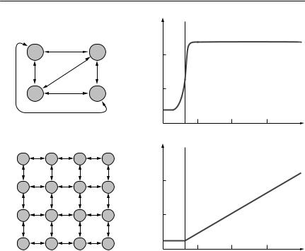
The methods of molecular genetics are increasingly providing useful data for estimating ecological parameters, particularly for spatial models. At the coarsest level of resolution, strong genetic differentiation between two or more subpopulations can be used to show that they function as independent breeding stocks. At a somewhat finer level of resolution, genetic data may provide information on the nature of the structuring of subpopulations. For example, some patterns of genetic variation suggest that subpopulations are connected according to an ‘island’ model (similar to a classical metapopulation or patch model), whereas other patterns suggest that subpopulations are connected according to a ‘stepping-stone’ model (similar to a lattice model). These models and the associated patterns of genetic variation are shown in Figure 7.5. The extent of genetic differentiation between populations is sometimes used to estimate the number of migrants exchanged per generation, but, as will be seen below, this relies on simplifying assumptions, which are liable to make such estimates inaccurate. A very recent and exciting development is to use high-resolution information about individuals’ genotypes to identify migrant individuals directly. This should enable much more accurate estimation of migration rates than has been possible in the past.
This book is not the place to go into the details of collecting and processing
S P A T I A L P A R A M E T E R S 197
FST
(a) |
(b) |
Distance |
|
|
FST |
(c) |
(d) |
Distance |
Fig. 7.5 Population structure and genetic divergence. In each case, lines with arrows represent equal rates of migrant exchange between patches (circles). Mating is assumed to be random within patches. (a) An island model. This is similar to an ecologist’s classic metapopulation model. (b) The expected relationship between the distance apart samples are taken and FST for an island model. The vertical dashed line is the patch size.
(c) A stepping-stone model (in this case, two-dimensional). This is similar to an ecologist’s lattice model. (d) The expected relationship between the distance apart samples are taken and FST for a stepping-stone model. The vertical dashed line is the patch size. Note that it may be difficult to discriminate between the relationships between genetic divergence and geographic distance in (a) and (b), given sampling error in the estimation of genetic divergence. This will be particularly so if the patch size is not known a priori.
genetic samples. Excellent reviews of the range of techniques available can be found in Hillis et al. (1996) or Parker et al. (1998). A summary of some of the available techniques and their potential applications is provided in Table 7.1.
Genetic data can potentially provide information on gene flow between subpopulations or through continuous space. This may not necessarily be the same thing as migration or movement of individuals. The classic method of estimating gene flow (Slatkin, 1985; 1987; Slatkin & Barton, 1989) is via the statistic FST. FST was originally defined by Wright (1951) as the component of the overall inbreeding coefficient F in a subdivided population that can be attributed to population subdivision. A simple conceptual definition is provided by Slatkin and Barton (1989):
Table 7.1 Molecular genetic methods and spatial parameters. For all but the first two methods, it is possible to use PCR, enabling data to be obtained from very small amounts of genetic material. Modified from Moritz and Lavery (1996), Jarne and Lagoda (1996) and Parker et al. (1998)
Method |
Genotype |
Allele |
Allele |
Ease of use/cost |
Applications |
Limitations |
|
freqs |
freqs |
genealogy |
|
|
|
|
|
|
|
|
|
|
Allozyme electrophoresis |
Yes |
Yes |
No |
Straightforward, cheap |
Good for population |
Low levels of polymorphism in |
|
|
|
|
|
structure, if enough |
many populations. May be subject to |
|
|
|
|
|
polymorphism |
selection |
Multilocus minisatellite |
No |
No |
No |
Cheap for a |
Excellent for identifying |
Relatively poor for population |
VNTRs ‘DNA fingerprints’ |
|
|
|
DNA technique. |
individuals |
structure. As many loci scored |
|
|
|
|
Analysis is tricky |
|
simultaneously, genotypes cannot |
|
|
|
|
|
|
be determined. |
Mitochondrial RFLPs |
Yes |
Yes |
Yes |
Relatively |
Good for population |
Entire MtDNA functions as a single |
|
|
|
|
straightforward |
structure. Mutation rate |
locus. Only maternally inherited. |
|
|
|
|
|
(and hence polymorphisms) |
Cannot identify individuals |
|
|
|
|
|
greater than most nuclear |
|
|
|
|
|
|
DNA loci |
|
Nuclear RFLPs |
Yes |
Yes |
Yes |
Somewhat more |
Good for overall population |
Amount of available polymorphism |
|
|
|
|
difficult than MtDNA |
structure |
may be limited |
Single locus |
Yes |
Yes |
Yes |
Relatively expensive. |
Excellent for identifying |
High initial setting-up costs for |
microsatellite VNTRs |
|
|
|
Primers must often be |
individuals |
working on a new species |
|
|
|
|
specially developed |
Sufficient resolution for |
|
|
|
|
|
|
assignment tests |
|
RAPDs |
No |
Yes |
No |
Method |
Potentially good both for |
Methods of analysis and |
|
|
|
|
straightforward, |
population structure and |
interpretation are not yet clearly |
|
|
|
|
analysis tricky |
individual identification |
established |
Sequences |
Yes |
Yes |
Yes |
Currently expensive |
Excellent for historical |
Costs and resulting small sample |
|
|
|
|
and time-consuming |
ecology |
sizes possibly make method not |
|
|
|
|
|
|
optimal for current population |
|
|
|
|
|
|
structure or for identifying |
|
|
|
|
|
|
individuals |
|
|
|
|
|
|
|
MtDNA, mitochondrial DNA; RAPD, random amplified polymorphic DNA; RFLP, restriction fragment length polymorphism; VNTR, variable number of tandem repeats.
7 R E T P A H C 198

|
|
|
|
S P A T I A L P A R A M E T E R S |
199 |
|
= |
f0 |
− U |
|
|
FST |
|
|
, |
(7.5) |
|
1 |
|
||||
|
|
− U |
|
||
where f0 is the probability of identity by descent of two alleles chosen at random from a single subpopulation (deme) and U is the probability of identity by descent of two alleles chosen at random from the entire population. Thus, if a population is not subdivided, FST = 0, and FST increases with population subdivision. In an infinite island model without mutation or selection, Wright (1951) showed that
FST |
≈ |
|
1 |
, |
(7.6) |
|
|
||||
|
1 |
+ 4Nm |
|
||
where Nm is the number of gametes (not individuals!) migrating into each patch per generation, made up from the probability that each gamete is a migrant m and the effective population size N. The first and most obvious point to emerge from eqn (7.6) is that, under this model, it does not take much migration (about one individual per generation) to prevent significant genetic differentiation. Further, it appears that, by using eqn (7.6) it may be possible to estimate the number of migrants per generation between populations, given
an estimate of FST.
Equation (7.6) is based on a highly idealized model, which has an infinite number of subpopulations of equal size, exchanging migrants equally with every other subpopulation, and with no selection or mutation occurring. Quite clearly, these are unrealistic assumptions, but Slatkin and Barton (1989) review simulations suggesting that the result in eqn (7.6) applies reasonably well in the face of mutation rates less than the migration rate, in cases where there are several (rather than infinite) subpopulations, where populations are connected via a stepping-stone model rather than an island model, and even where there is selection, provided the selection coefficient is less than the migration rate. Some other authors, however (e.g. Weir, 1996; or Bossart & Prowell, 1998) are less confident about the applicability of the equation in real situations.
A second issue is that eqn (7.5) is a conceptual definition, and cannot be used to estimate FST directly from data. There are several ways that FST can be estimated, and somewhat confusingly, these are often represented with symbols other than FST. There is a review of these methods in Weir (1996). Most people are likely to use a packaged program such as FSTAT (Goudet, 1995) to calculate them.
Other approaches to estimating Nm from genetic information do not use FST. One approach is to assume that the distribution of allele frequencies follows a beta distribution, one of the parameters of which is Nm, and then to estimate Nm by maximum likelihood (Slatkin & Barton, 1989). This approach, however, appears to overestimate Nm unless a very large number of subpopulations is

200 C H A P T E R 7
sampled. The rare alleles or ‘private alleles’ method uses the mean frequency of alleles that are present in only one population to estimate gene flow, following the intuitive idea that there will be more such alleles if there is little gene flow than if gene flow is substantial. However, it appears that this method is probably not as useful as those based on FST (Slatkin & Barton, 1989).
An entirely different approach to the use of genetic data for estimating migration rates has recently been developed. The idea is to use high-resolution genetic methods to identify, as probable migrants, individuals whose genotype is more typical of a neighbouring population than the population in which they were recorded. The raw data necessary are simply a set of genotypes, based on a number of loci, from individuals in more than one population. It is not essential that each genotype is unique, but the more different genotypes there are in the data set, the more powerful the method will be. The genetic data have usually been derived from single-locus microsatellites, but allozymes, RAPDs, or combinations of all these can also be used (Waser & Strobeck, 1998).
The method is based on an extremely simple ‘assignment test’, which is used to assign an individual to the population to which it is most similar, on the basis of its genotype. The test follows these steps (Waser & Strobeck, 1998):
1 Remove the test individual’s genotype from the population in which it was found, and then estimate allele frequencies at each locus using the remaining individuals sampled from that population. These frequencies can be repres-
ented as pil, pjl, . . . for alleles i,j, . . . at locus l.
2 At any particular locus l, the likelihood of the test individual having the genotype it was observed to possess, given the population’s allele frequencies, is then p2il if it was homozygous for allele i, and 2pil pjl if it was heterozygous for alleles i and j.
3 The log-likelihood of the test individual possessing its overall genotype, given the population’s observed allele frequencies, is then simply the sum of the log-transformed individual likelihoods.
4 Repeat the above steps for each of the putative populations to which the individual may belong.
5 Assign the individual to the population in which it has the highest likelihood of occurrence.
It is implicit in step 2 that each population is in Hardy–Weinberg equilibrium, and implicit in step 3 that there is no linkage disequilibrium. There is a problem if an allele possessed by the individual being assigned is not present in a particular sample from a test population. This would cause the probability of the individual being assigned to that population to be calculated as zero, making the log-likelihood infinitely small. If the allele were indeed absent from the test population, this would be correct. However, as the data are samples from the populations, and not entire populations, there is a finite

S P A T I A L P A R A M E T E R S 201
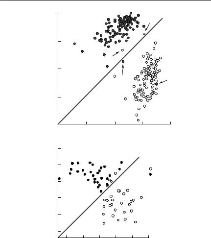
probability that a particular allele is present in the population, but not the sample. An appropriate work-around is to assign the missing allele a very low frequency such as 1/2N, where N is the number of individuals sampled from the test population. Figure 7.6 shows examples applying this method.
It should be obvious that this method may detect animals as ‘immigrants’ that are not immigrants themselves, but the descendants of immigrants. If there is random mating within each population, as is assumed by the method, immigrant genotypes should get diluted fairly rapidly. However, the same basic approach has been used, with reasonable power, to detect immigrant human genotypes in populations up to about the second generation (Rannala & Mountain, 1997).
There is great potential in these microsatellite-based methods to investigate dispersal over ecological time scales, rather than over evolutionary time scales, which most other genetic methods operate on. Further research is required to determine the extent to which this potential may be realized. Individuals can only be unequivocally identified as migrants if they are clearly genetically distinct from the population in which they are found, but it may be that even modest levels of gene flow are sufficient to prevent enough genetic differentiation occurring to be able to make genetic distinctions between individuals from different populations. For example, the polar bear populations in Fig. 7.6(b) are separated by several thousand kilometres, yet several individuals lie very close to the assignment boundary between the populations.
Even if individual dispersers cannot clearly be identified, assignmentbased methods may still be valuable in making inferences about dispersal. For example, using microsatellite data, Favre et al. (1997) found that female shrews were less likely to be assigned to the population in which they were found than were males. This matched the results of an extensive mark– recapture program showing that dispersal was strongly female-biased.
Metapopulations
A metapopulation is a population of subpopulations, separated in space from each other, and with limited movement between subpopulations. Such a broad definition could apply to almost all species. The ‘classic’ metapopulation model, developed by Levins (1969; 1970), is, however, much more restrictive. It assumes a large number of identical, discrete habitat patches, connected by migration. Patches are scored as either occupied or vacant, with the population density on each patch not being considered. The single variable modelled is the proportion of occupied patches P, and this is assumed to be influenced by two parameters only: c, the colonization rate; and e, the extinction rate. Colonization is assumed to occur at a rate proportional to the product of the proportion of occupied patches (sources of colonists) and the proportion of
202 C H A P T E R
Log-likelihood from population B
7
–2
–6
–10
–14
|
–18 |
–14 |
|
–10 |
|
–6 |
–2 |
(a) |
|
Log-likelihood from population A |
|
||||
|
4 |
|
|
|
|
|
|
(WH) |
6 |
|
|
|
|
|
NB |
|
|
|
|
|
|
||
|
|
|
|
|
|
WH |
|
8 |
|
|
|
|
|
|
|
–Log(frequency) |
|
|
|
|
|
|
|
10 |
|
|
|
|
|
|
|
12 |
|
|
|
|
|
|
|
|
|
|
|
|
|
|
|
|
14 |
|
|
|
|
|
|
|
14 |
12 |
10 |
8 |
6 |
4 |
|
(b) |
|
–Log(frequency) (NB) |
|
|
|||
Fig. 7.6 Assignment tests. (a) An example based on simulated data from Waser and Strobeck (1998). The simulated populations have eight loci with 12 alleles each. Each population consists of 100 individuals, and the migration rate is 0.005 (one individual every second generation). Genotypes actually from population A are shown with open circles, whereas those from B are shown with closed circles. Genotypes above the 45˚ line have a higher likelihood of belonging to population B than to population A. Four individuals (arrowed) are misaligned. The B individual at the right-hand side of the A cluster is in fact an immigrant. (b) An example using real data on polar bears from Paetkau and Strobeck (1998). The likelihood of bears’ genotypes coming from Western Hudson Bay (WH) or
the North Beaufort Sea (NB) is shown. There is clear genetic separation between the two populations, although four North Beaufort Sea animals are assigned wrongly to Western Hudson Bay. As these are very close to the 45˚ line, they do not have a much greater likelihood of belonging to one population than the other, and they cannot be inferred to be immigrants. Based on eight microsatellite loci with four to nine alleles per locus (Paetkau & Strobeck, 1998). Note that polar bears have particularly low levels of genetic variation when assayed with allozyme electrophoresis or mitochondrial DNA.

S P A T I A L P A R A M E T E R S 203
vacant patches (available targets). Extinction occurs at a constant rate per occupied patch. These assumptions lead to the following simple equation to describe the rate of change in the proportion of occupied patches:
dP |
= cP(1 − P) − eP |
(7.7) |
|
||
dt |
|
|
This equation is identical in structure to the logistic equation. Its extreme simplicity makes it very valuable for drawing very general conclusions about populations divided into discrete patches (see, for example, Hanski, 1997a). There is little value, however, in attempting to apply such a general model in any specific case, and therefore little point in discussing estimation of the colonization and extinction parameters.
Some authors have questioned how common metapopulations are in the real world (e.g. Harrison, 1994). Certainly, no real population will meet the assumptions of this highly stylized model exactly. There is little value in applying the model to species that move between patches so frequently that ‘extinction’ on a patch is a meaningless term, and there is equally little point in applying it in situations where movement between patches is so rare that it has no appreciable impact on population dynamics.
The crucial property of a system that makes the metapopulation paradigm useful is that the proportion of occupied patches should be an adequate descriptor of the overall state of the population. If the population density per patch and its frequency distribution are needed to describe the population adequately, then it is a spatially subdivided population, but not one to which the classic metapopulation paradigm applies easily. Hanski (1997a) provides four conditions that should be satisfied if a metapopulation approach is likely to prove useful:
1 The suitable habitat occurs in discrete patches which may be occupied by local breeding populations.
2 Even the largest local populations have a substantial risk of extinction. 3 Habitat patches must not be too isolated to prevent recolonization.
4Local populations do not have completely synchronous dynamics.
If the assumptions of the classical metapopulation model are relaxed a little,
so that patches may differ in extinction probability according to size, and in recolonization probability according to location, a model can be produced that is sufficiently realistic to be parameterized. In at least some cases, such models also appear to have real conservation applications. Hanski (1994; 1997b) has developed this idea in some detail, and has named it the ‘incidence function’ approach.
There are many models in the literature, described as ‘metapopulation models’, that do not satisfy the above criteria fully (for example, Possingham et al., 1992b; 1994; Lindenmayer and Lacy, 1995a; 1995b). To debate whether

204 C H A P T E R 7
these are ‘real’ metapopulation models is fairly sterile. However, to parameterize them, it is necessary to have information at the level of the individual patch on migration rates, birth and death rates, etc. This requires approaches discussed earlier in this chapter, and in previous chapters. From the perspective of parameterization, a metapopulation model is one that can be parameterized by estimating patch-specific extinction and colonization rates.
Incidence function models
The incidence function approach developed by Hanski (1994) offers the promise of a metapopulation model realistic enough to be useful for quantitative prediction of the extinction probability of a metapopulation, but simple enough to be parameterized. I will therefore discuss the model and parameter estimation for the model in some detail.
The model expands the classic Levins model by including information on the spatial configuration of patches and patch sizes. Extinction of the study species on a patch is allowed to be a function of patch area, and colonization probability is allowed to be a function of patch isolation. Only presence or absence of the study species is used in the analysis. If patch i is vacant in year t, it has a probability Ci of being recolonized by year t + 1. If patch i is occupied in year t, it has a probability Ei of being vacant by year t + 1.
Given a large number of patches, differing in area and isolation, and plausible functional forms relating extinction and colonization to these two variables, it is possible, in principle, to estimate parameters for Ci and Ei directly. The logical approach would be some form of logistic regression (see Chapter 2), and it has been used by Sjögren Gulve (1994) for this purpose. The difficulty with this approach is that a substantial time series of extinctions and colonizations is required (see Hanski, 1997b). Hanski cleverly circumvents the problem by instead estimating the incidence Ji, or long-run probability that patch i is occupied, as a function of patch size and isolation. Together with some additional information, these estimates can then be used to estimate the extinction and colonization rates, permitting the metapopulation process to be simulated.
Provided the system is in stochastic steady state (that is, the mean number of occupied patches is neither increasing nor decreasing), Ji is related to the extinction and colonization probabilities by
Ji |
= |
|
Ci |
(7.8) |
|
Ci |
+ Ei |
||||
|
|
|
(Hanski, 1994). Given the steady-state assumption (which may well be a problem, if the objective is to model a population that is in decline), incidence can be modelled from a single snapshot of presence and absence on a large number of patches. As is the case with direct estimation of extinction and

|
|
S P A T I A L P A R A M E T E R S 205 |
Table 7.2 Parameter and variable definitions for Hanski’s incidence function |
||
metapopulation model |
|
|
|
|
|
Parameter |
Description |
Comments |
|
|
|
Ci |
Probability of colonization of patch i |
|
|
in a single time interval |
|
Ei |
Probability of extinction of the population |
|
|
on patch i in a single time interval |
|
Ji |
The long-term probability of patch i |
Defined as ‘incidence’ by Hanski |
|
being occupied |
|
Ai |
Area of ith patch |
Obtained directly from data |
xParameter describing how extinction
scales with patch area
eParameter describing the minimum patch
|
size on which a population can persist |
|
Mi |
Number of migrants arriving on patch i in |
|
|
a single time interval |
|
y |
Half-saturation parameter of the sigmoid |
Number of migrants per time |
|
relationship between number of |
interval that results in a |
|
migrants and probability of successful |
probability of 0.5 of successful |
|
colonization |
colonization |
Si |
Isolation of patch i |
Depends on distance to other |
|
|
patches, their size, and |
|
|
occupancy. Obtained from data, |
|
|
given assumption of steady |
|
|
state, and an independent |
|
|
estimate of the parameter α |
βParameter relating isolation to
|
number of migrants |
|
dij |
Distance between patches i and j |
Obtained directly from data |
α |
Parameter describing rate at which |
|
|
isolation increases with distance |
|
y′ |
Parameter combination linking |
y′ = (y/β )2 |
|
probability of colonization to isolation |
|
|
|
|
colonization rates, it is necessary to assume plausible forms for the dependence of extinction and colonization on patch size and isolation. These are then substituted into eqn (7.8) to estimate the parameters themselves. Depending on the biology of the species concerned, a number of possible functional forms can be used.
The following description of the estimation procedure is based on Hanski (1997b), unless explicity stated otherwise. Table 7.2 summarizes the parameter and variable definitions.
Equation (7.8) should first be modified slightly by the addition of a ‘rescue effect’. Colonists will arrive at a patch when it is occupied as well as when it is vacant. A patch with a high colonization rate should have a lowered extinction rate, as colonists will sometimes prevent extinction by arriving at a patch in a year when the patch population would otherwise have become extinct, as well as by recolonizing a patch once extinct. The incidence is thus

206 C H A P T E R 7
Ji |
= |
|
Ci |
|
= |
|
Ci |
. |
(7.9) |
Ci |
+ Ei(1 |
|
|
+ Ei − EiCi |
|||||
|
|
− Ci ) Ci |
|
|
|||||
A plausible form for the extinction probability Ei is
Ei |
= min 1, |
|
, |
(7.10) |
|
||||
|
|
Ax |
|
|
|
|
i |
|
|
here Ai is the area of the ith patch, and x is a parameter describing how extinction probability scales with patch area. The parameter e essentially determines the minimum patch size on which the species has any chance of surviving: if
Ai ≤ e1/x, |
(7.11) |
extinction is certain in one time period.
Colonization is harder to model plausibly. It will depend in some way on the mean number of immigrants Mi arriving at the ith patch per unit of time, which will in turn depend on both the distances to and sizes of nearby patches. A possible relationship between Mi and Ci is
|
= |
|
M2 |
|
|
|
C i |
|
i |
. |
(7.12) |
||
y2 |
+ M2i |
|||||
|
|
|
|
This generates an S-shaped curve, so that small numbers of migrants have a very small chance of colonizing a patch, but large numbers of migrants are almost certain to do so. The parameter y tunes the shape of this curve. Other functional forms may be appropriate in some contexts.
The next problem is an appropriate form for Mi. Hanski suggests
Mi = βSi , |
(7.13) |
where β is a parameter to be estimated, and Si is a measure of the isolation of patch i. In Hanski’s model,
Si = Σpj Aj exp(−αdij). |
(7.14) |
j≠i |
|
Here, pj equals 0 for empty patches, and 1 for occupied patches, dij is the distance from the ith to jth patches, and α is a parameter to be fitted. The model is thus assuming that the number of migrants a patch contributes to another is proportional to the product of the donor patch area and a negative exponential function of the distance between patches (following the dispersal model of eqn (7.1)). At a cost of an additional parameter, colonization can alternatively be made to scale as a power of Ai.
To make this workable, it needs to be further assumed that Mi is constant at steady state, so that the observed pi distribution can be used to estimated the model parameters. In reality, even at stochastic steady state, the pi set would

S P A T I A L P A R A M E T E R S 207
change as individual patches winked on and off (thus causing the number of migrants to each patch to change).
Note, that by combining eqns (7.12) and (7.13), eqn (7.12) can be written as
C = |
S2 |
|
(7.15) |
|
(y/β)2 |
+ S2 |
|||
|
|
and thus only the combination y′ = (y/β)2 needs to be estimated. Having made these assumptions, eqn (7.9) becomes
|
|
ey′ |
|
J = 1 |
+ |
|
. |
|
|||
|
|
S2 Ax |
|
Equation (7.16) may be written as
Ji = [1 + exp[ln(e y′) − 2ln Si − xln Ai]−1
and, furthermore,
J
ln = −ln(ey′) + 2ln S + xln A .
1 − J
(7.16)
(7.17)
(7.18)
This is now a standard logistic regression, meaning that given a series of observed Ji, Ai and Si, standard packages can be used to estimate the parameter x, and the parameter combination −ln(e y′), using 2ln Si as an offset (see Crawley, 1993). Two problems remain. First, Si does not consist solely of observable quantities: it includes the unknown parameter α. Second, e and y′ cannot be disentangled, but an estimate of e itself is needed in eqn (7.10) if the metapopulation model is to be iterated.
Hanski (1994) suggests that α should be estimated from independent movement data. For example, α could be estimated as the decay parameter of eqn (7.1), using an experiment like that described by Hill et al. (1996). Note that it is not necessary to estimate the number of migrants dispersing to particular distances from a patch of area A, only the way in which the number of dispersers declines with distance from the source population. Alternatively, an iterative nonlinear method could be used to estimate this parameter, but that would considerably complicate things. Hanski (1994) asserts that the results of an incidence function simulation are not strongly dependent on the value of α that is used.
Hanski (1997b) suggests that e should be estimated from the size of the threshold patch size, beyond which extinction is certain. Using eqn (7.11), this will give an independent estimate of e. The area of the smallest occupied patch, A0, could be used in the absence of other data. Following eqn (7.11),
e = Ax0. |
(7.19) |
An example of an application of this model is shown in Box 7.1.
208 C H A P T E R 7
Box 7.1 Using the incidence function approach to predict the consequences of habitat destruction in an endangered butterfly
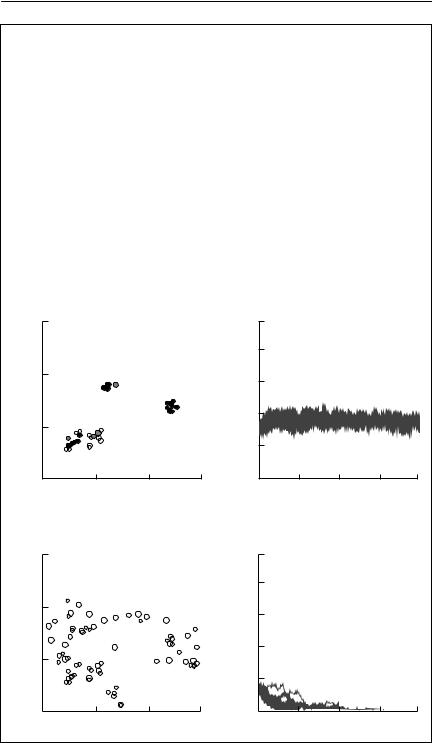
This example is based on Wahlberg et al. (1996). The false fritillary butterfly (Melitaea diamina) is endangered throughout most of its range in Europe. It requires habitat patches consisting of moist meadows where its larval host plant is present. Wahlberg et al. (1996) surveyed its only well-known metapopulation in Finland, recording the distribution and areas of habitat patches shown in (a) below. Solid circles represent occupied patches and open circles are unoccupied patches of suitable habitat (94 patches in total, 35 occupied). Circle diameters are proportional to patch areas (ranging from 0.005 to 4 ha).
As this is an endangered species occupying a relatively small number of patches, it is difficult to use data for the species itself to estimate parameters for the incidence function model. Hanski (1994) estimated parameters for the related butterfly, Melitaea cinxia, in 1600 habitat patches in Finland. These were used to attempt to predict the dynamics of the endangered species. The parameters used were:
x |
ey ′ |
e |
α |
b* |
A0 |
0.952 |
0.158 |
0.010 |
1.0 |
0.5 |
79 m2 |
|
|
|
|
|
|
*In this example, a minor variant of eqn (7.12) was used, in which the effect of patch area on colonization was proportional to Abi.
With these parameters, the predicted incidence of patch occupancy is as shown below in (b), where the depth of shading is proportional to the
Distance (km)
30
20
10
30
20
10
0 |
10 |
20 |
30 |
0 |
10 |
20 |
30 |
(a) |
Distance (km) |
|
(b) |
Distance (km) |
|
||
continued on p. 209
S P A T I A L P A R A M E T E R S 209
Box 7.1 contd
probability of the patch being occupied. The close correspondence to the observed occupancy is obvious.
The model was then iterated to investigate the consequences of various patterns of habitat destruction. In (a) 47 patches (representing 55% of the total habitat area) were destroyed. These are shown as crosses. Note that the destroyed patches are around the periphery of the patch network. The consequences are shown as the results of 10 replicate simulations over 400 time intervals. This pattern of destruction is not predicted to lead to extinction of the entire metapopulation. In contrast, (b) shows the consequences of destroying just 15 patches (44% of the total area) that are in the centre of the patch network. It is clear that this pattern of destruction is predicted to lead to extinction of the metapopulation over a short time horizon.
Distance (km)
(a)
30
20
10
0
|
|
|
|
|
|
|
|
|
|
(P) |
1.0 |
|
|
|
|
|
|
|
|
|
|
|
|
|
|
|
|
|
|
|
|
|
|
|
|
|
|
|
|
|
|
occupied |
0.8 |
|
|
|
|
|
|
|
|
|
|
|
|
|
|
|
|
|
|
|
|
|
|
x |
x |
|
|
|
|
|
|
|
|
|
|
|
|
|
|
x |
|
|
|
|
|
|
|
|
|
|
|
|
|
x x |
xx |
|
x |
x |
x x |
x |
|
|
patches |
0.6 |
|
|
|
|
|
xx |
x x |
x |
x |
|
x |
|
|
|
|
|
|||||
x |
|
|
x |
|
|
|
|
|
|
|
|
||||
|
|
x x |
|
|
|
|
x |
|
|
|
|
|
|
||
|
|
x |
x |
|
|
|
|
|
x |
|
|
|
|
|
|
|
|
|
|
|
|
|
|
|
|
|
|
|
|
|
|
|
xx |
|
|
|
x |
x |
x |
x |
of |
0.4 |
|
|
|
|
|
|
x |
xx |
|
|
|
|
|
|
|
|
|
||||
|
|
|
|
x x |
|
|
|
xxxxx |
Fraction |
|
|
|
|
|
|
|
|
|
|
|
|
|
|
|
0.2 |
|
|
|
|
||
|
|
|
|
|
xxx |
|
|
|
|
|
|
|
|
|
|
|
|
|
|
|
|
|
|
|
|
|
|
|
|
|
|
|
|
|
|
|
x |
|
|
|
|
|
0.00 |
|
|
|
|
|
|
|
|
10 |
|
20 |
|
|
30 |
|
100 |
200 |
300 |
400 |
|
|
|
|
|
Distance (km) |
|
|
|
|
|
|
Time units |
|
|
||
Distance (km)
(b)
30 |
|
|
|
|
20 |
|
x |
|
|
x |
x |
x |
|
|
|
|
|||
|
|
|
x |
|
10 |
x |
x |
x |
x |
|
x |
|
||
|
|
|
|
x |
0 |
|
10 |
20 |
30 |
|
|
Distance (km) |
|
|
Fraction of patches occupied (P)
1.0
0.8
0.6
0.4
0.2
0.00 |
100 |
200 |
300 |
400 |
|
|
Time units |
|
|

210 C H A P T E R 7
Diffusion models
Diffusion models are probably the most abstract form of spatial model. Space is considered to be continuous, rather than a series of patches or cells. The approach dates at least back to Skellam (1951). A recent, brief review is provided by Hastings (1996), and a fuller treatment can be found in Murray (1989).
In two dimensions, the simplest possible diffusion model is
∂n |
= rn + |
1 |
|
∂2n |
+ |
∂2n |
|
|
|
|
|
s |
|
|
|
(7.20) |
|||
∂t |
2 |
∂x 2 |
∂x 2 |
||||||
|
|
|
|
|
|||||
|
|
|
1 |
|
2 |
|
(van den Bosch et al., 1992). Here, n is the population density at time t at a position in a two-dimensional plane defined by the coordinate pair (x1, x2), r is the intrinsic rate of growth and s is the diffusion constant. The model assumes that animals move randomly throughout life, at a constant rate that determines the diffusion coefficient s. In this simplest version of the diffusion model, the rate of spread s is the same in all directions, although this assumption can be relaxed fairly easily. Neither demographic parameters nor movement parameters depend on age or local population density.
The principal result from this simple model is that the square root of area occupied is predicted to increase as a linear function of time, with a rate coefficient
C = 2rs. |
(7.21) |
Surprisingly, this highly unrealistic model often fits observed data on area occupied as a function of time since release quite well, particularly after the initial stages (see Fig. 7.7). The most important general point to be gained from eqn (7.21) is that the rate of spread of an invading population is a function not only of the dispersal rate of individuals, but also of the intrinsic growth rate of the population.
Potentially, eqn (7.21) could be used directly to estimate the diffusion coefficient, given an observed rate of spread, and an estimate of the intrinsic rate of growth r (see Chapter 5). In reality, however, this approach is unlikely to be useful in many cases. The practical problem is usually one of predicting the rate of spread of an invasive species or genotype, and if the rate of spread is required to estimate the diffusion coefficient, this is begging the question. Equation (7.20) is a highly abstract model. In common with many of the abstract models discussed in this book, its parameters are compound entities that do not correspond closely to directly observable ecological quantities. It is difficult to estimate s directly from data, even if one is prepared to accept that the assumptions the model makes can reasonably be justified.
Square root of area occupied (x103 km)
4
3
2
1
1900 1920 1940 1960
S P A T I A L P A R A M E T E R S 211
8
7
6
5
4
3
2
1
0
1910 1920 1930 1940 1950 1960
(a) |
|
|
|
|
(b) |
|
|
|
km) |
6 |
|
|
|
5 |
|
|
|
|
|
|
|
|
|
|
||
|
|
|
|
|
|
|
|
|
3 |
|
|
|
|
|
|
|
|
(x10 |
5 |
|
|
|
4 |
|
|
|
|
|
|
|
|
|
|
||
occupied |
|
|
|
|
|
|
|
|
4 |
|
|
|
|
|
|
|
|
|
|
|
|
|
|
|
|
|
|
|
|
|
|
3 |
|
|
|
area |
3 |
|
|
|
|
|
|
|
|
|
|
|
2 |
|
|
|
|
of |
2 |
|
|
|
|
|
|
|
|
|
|
|
|
|
|
||
root |
|
|
|
|
|
|
|
|
1 |
|
|
|
1 |
|
|
|
|
Square |
|
|
|
|
|
|
||
|
|
|
|
|
|
|
||
0 |
|
|
|
0 |
|
|
|
|
|
1930 |
1940 |
1950 |
1940 |
1950 |
1960 |
1970 |
|
|
1920 |
|||||||
(c) |
|
Year |
|
(d) |
|
Year |
|
|
|
|
|
|
|
|
|
||
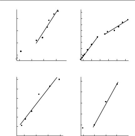
Fig. 7.7 Area occupied by invading species as a function of time since introduction:
(a)The collared dove (Streptopelia decaocto) introduced into Europe from Asia in about 1900.
(b)The muskrat (Ondatra zibethicus), escaped from a fur farm near Prague in 1905. A largescale trapping program commenced in about 1930. Two separate regression lines, up to, and after, 1930 are therefore shown. (c) The starling (Sturnus vulgaris), released in New York City in 1890/91. (d) The cattle egret (Bubulus ibis ibis), invaded the Americas in about 1930. From van den Bosch et al. (1992).
Van den Bosch et al. (1992) present a method to predict the rate of range expansion of a population, given demographic data and dispersal data for individuals. The method is based on an integral equation, details of which can be found in the above paper. In general terms, the model assumes that the population is age-structured, with constant age-specific fecundity and mortality rates. It derives a relationship between the number of births at time t at a particular point in space and the number of births in the past at all other possible positions. Dispersal is assumed to be independent for each individual, to have no particular preferred direction, and not to depend on either local

212 C H A P T E R 7
Table 7.3 Parameters for the van den Bosch et al. (1992) models of range expansion. In this table, i represents the age class; Mi represents age-specific fecundity; Li represents agespecific survivorship (the proportion of individuals surviving from the first census to census i); and li represents the midpoint of the age interval i. For dispersal data, it is assumed that n observations are available of individual dispersal distances dj. These are assumed to be records of distances moved between birth and adulthood for animals that disperse only as juveniles. For animals that disperse at a constant rate throughout life, the data available are likely to be distances moved between successive census intervals. This complicates the estimation of dispersal parameters (see van den Bosch et al. (1992) for details)
Parameter |
Parameter definition |
Estimation formula |
||||||||||||||
|
|
|
|
|
|
|
|
|
|
|
|
|
|
|
||
R0 |
Net reproductive rate |
\0 = ∑L M |
|
|
||||||||||||
μ |
Mean age of reproduction |
E = 1 ∑l L M |
|
|||||||||||||
|
|
|
|
|
|
|
|
|
|
|
|
|
|
|
||
|
|
|
|
|
|
|
|
|||||||||
|
|
|
|
R0 |
|
|
||||||||||
υ |
Variance in age of reproduction |
! = |
|
|
1 |
|
∑l 2L M − E2 |
|||||||||
|
|
\0 |
|
|||||||||||||
|
|
|
|
|
|
|
|
|
|
|
|
|
||||
σ 2r |
Variance of spatial distribution of recaptured animals |
|
|
|
|
|
∑d2j |
|
|
|||||||
|
|
ˆ 2 |
|
|
|
|
j |
|
|
|
||||||
|
|
σ r |
= |
|
|
2n |
|
|
||||||||
|
|
|
|
|
|
|
|
|
|
|||||||
γr |
Kurtosis of spatial distribution of recaptured animals |
@ |
= |
|
|
1 3 1 |
∑d |
4 − 3 |
||||||||
|
|
r |
|
|
F 4 |
|
8 |
|
n |
j |
j |
|||||
|
|
|
|
|
|
|
|
|
|
|
|
|
|
|
|
|
|
|
|
|
|
|
|
|
|
|
|
|
|
|
|
|
|
population density or the current position in space. These are quite restrictive assumptions.
Van den Bosch et al. (1992) develop various approximations that predict the rate of range expansion. In the simplest possible case, individual animals could be assumed to move randomly throughout life, with dispersal distance following a normal distribution. If this is the case, they show that eqn (7.21) represents the rate of expansion of the population, with r being the usual intrinsic rate of growth, and s being the rate at which the variance of dispersal distance increases with age. Given a large set of data giving distance to which individuals had dispersed from their natal position, as a function of age, it would be possible to estimate the variance of the dispersal distance as a function of age. If dispersal were indeed continuous, then the relationship between that variance and age would be a straight line passing through the origin, and the slope of that line would estimate the parameter s in eqn (7.21). Unfortunately, such data are rarely available, and if they were, it is unlikely that there would be a simple linear relationship between the variance of dispersal distance and age. Few animals move at random at a constant rate throughout life. More reasonable assumptions are required in practice.
Table 7.3 defines parameters for species demography and dispersal that can

S P A T I A L P A R A M E T E R S 213
be used to estimate the rate of population expansion. Using these definitions, van den Bosch et al. (1992) show that, for relatively slowly reproducing species (R0 < 1.5),
C ≈ |
σ r |
2ln R0 . |
(7.22) |
|
μ |
||||
|
|
|
Comparing eqn (7.22) with eqn (7.21), it is possible to identify the approximations
r ≈ |
ln R0 |
(7.23) |
||
μ |
||||
|
|
|||
and |
|
|||
s = |
σ 2 |
|
||
r |
. |
(7.24) |
||
|
||||
|
μ |
|
||
For more rapidly reproducing species (1.5 < R0 < 7), van den Bosch et al. suggest the following approximation:
|
σ |
|
|
|
υ |
2 |
1 |
|
|
|
|
|
|
|
|
|
|
|
|
|
|
|
|||
C ≈ |
|
2ln R |
1 |
+ |
|
− |
|
|
γ ln R |
. |
(7.25) |
|
|
|
|
||||||||||
|
μ |
0 |
|
|
μ |
|
12 |
0 |
|
|
||
|
|
|
|
|
|
|
|
|
|
|
|
|
This should be a reasonable approximation provided υ/μ < 0.06, and if dispersal occurs only in juveniles. If adults move as well, a more complicated approximation is needed. For details, see van den Bosch et al. (1992).
The relationship between these predicted rates of spread and observed rates of spread is shown in Fig. 7.8 for some vertebrate species. The correspondence between observed and predicted rates is encouraging. It is not possible to determine whether the discrepancies are a result of failures in the model assumptions or inaccuracies in the input data. Van den Bosch et al. (1992) used literature values for dispersal distances. As has been discussed earlier in this chapter, such data are likely to contain a variety of biases and inaccuracies. As the equations rely on the second and fourth moments of the distribution of dispersal distances, any inaccuracies are likely to be magnified. It is interesting to note that the more elaborate eqn (7.25) appears, for these examples at least, to provide somewhat more accurate predictions than the far simpler eqn (7.22), but the difference is not dramatic.
In most of the examples shown in Fig. 7.8, the actual rate of spread is underestimated by the simple model. A possible explanation is that rare, long-distance dispersal events increase the rate of spread. Hengeveld (1994) discusses this problem, together with some partial solutions. Rare events are always hard to detect, so it is unlikely that there are complete solutions. Another limitation of the model is that density dependence is not included.
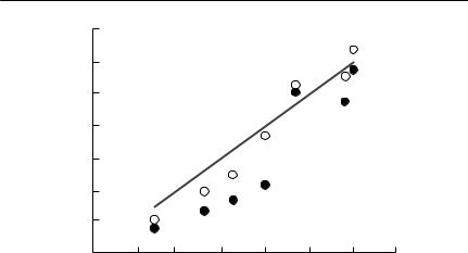
214 C H A P T E R 7
|
200 |
|
|
|
|
|
|
|
|
104 |
|
|
|
Collared dove |
|
|
|
|
|
|
|
|
Cattle egret |
|||
|
|
|
|
|
|
|
||
|
54 |
|
|
|
|
|
|
|
C |
|
|
|
|
|
|
Starling |
|
Predicted |
28 |
|
|
|
|
|
|
|
14 |
|
|
|
|
|
|
|
|
|
|
|
|
|
|
|
|
|
|
7 |
|
|
|
|
House sparrow, Europe |
|
|
|
|
|
|
|
|
|
|
|
|
|
|
|
|
House sparrow, USA |
|
|
|
|
4 |
|
|
Musk rat 1900–30 |
|
|
|
|
|
|
Musk rat 1930–60 |
|
|
|
|
||
|
2 |
4 |
7 |
14 |
28 |
54 |
104 |
200 |
Observed C
Fig. 7.8 The observed rate of spread of some vertebrates compared with their predicted rate of spread. Data points represented by black circles used expected rates of spread calculated from eqn (7.22), whereas open circles show expected rates calculated from eqn (7.25). If predictions were perfect, all points would fall on the 45˚ line. From data in van den Bosch
et al. (1992).
Population growth will inevitably decline as local density increases, although it may be that direct density dependence is not of crucial importance when considering the initial stages of population spread. To some extent, an increased propensity to disperse at high densities may compensate for lower population growth. Alternatively, there may be inverse density dependence (an Allee effect) at very low densities: the rare long-distance dispersers may have difficulty finding mates. This may have a significant impact on the rate of spread of an invader (Kot et al., 1996; Veit & Lewis, 1996). Some approaches that may be helpful for ‘fat-tailed’ distributions (that is, those in which there are some very long-distance dispersers) are outlined by Kot et al. (1996).
Summary and recommendations
1 An unbiased representation of the frequency distribution of dispersal distances is difficult to obtain. The distribution is almost always highly skewed, with a few individuals moving very long distances. Some methods, such as mark–recapture studies in a finite study area, will underestimate longdistance dispersal. Others, such as band recovery, tend to overestimate it. Using radiotelemetry to follow individuals is expensive, but is the best way to obtain unbiased data.
2 The probability distribution of dispersal distance of propagules from a parent organism is often estimated by placing collectors of a given area at

S P A T I A L P A R A M E T E R S 215
different distances and directions from the parent. If you use this approach, it is important to recognize that a uniform probability distribution of dispersal distance leads to the number of propagules per unit area declining as the square of distance, and to correct accordingly.
3 Formal mark–recapture methods can be used to estimate migration rates between subpopulations or habitat patches, but it is difficult to differentiate between survival and migration rates. Recapture rates must be reasonably high for these approaches to be useful.
4 Molecular genetic data are useful for determining whether there is gene flow between populations, and can shed light on the spatial pattern of gene flow. However, a small amount of migration is sufficient to prevent genetic differentiation. Methods based on statistics such as FST are most useful over an evolutionary, rather than an ecological, time scale. They are relatively poor at estimating the amount of migration in ecological time. The recent development of ‘assignment tests’ holds promise for measuring ecologically relevant migration rates.
5 Many spatially divided populations are described as ‘metapopulations’. For parameter estimation, a metapopulation is a system that can adequately be characterized by describing patches as ‘occupied’ or ‘vacant’, without using information about the population size or structure on each patch. The parameters that then need to be estimated are patch-specific probabilities of extinction and colonization.
6 The incidence function approach has potential to be realistic enough to be useful, but simple enough to be parameterized. How widely applicable it is remains to be seen.
7 Diffusion models for invading species are very abstract, but their key prediction that the square root of area occupied should be a linear function of time since invasion is often surprisingly accurate. To use these models predictively, it is necessary to be able to estimate the diffusion coefficient from demographic data. This is not easy. Table 7.3 and eqns (7.22) to (7.25) provide some suggestions on how to proceed, but these require an accurate description of the probability distribution of individual dispersal distances, up to the fourth moment (kurtosis).