So far we have restricted our attention to the case of a positive cosmological constant. While this seems to be the most relevant to the evolution of our universe, cosmologies with negative cosmological constant are also interesting. We leave their exploration to the exercises.

Einstein introduced the cosmological constant in order to allow his equations to have a

˙ =

static solution, R 0. He did not know about the Hubble flow at the time, and he followed the standard assumption of astronomers of his day that the universe was static. Even in the framework of Newtonian gravity, this would have presented problems, but no-one seems to have tried to find a solution until Einstein addressed the issue within general relativity.

˙ =

We have to do more than just set R 0 in Eq. (12.54); we have to guarantee that the

˙

solution is an equilibrium one, that the dynamics won’t change R, i.e. that the universe is at a minimum or maximum of the ‘potential’ we discussed earlier. We show in Exer. 20, § 12.6 that the static solution requires

1

ρ = 2 ρ0.

For Einstein’s static solution, the dark energy density has to be exactly half of the matter energy density. We shall see below that in our universe the measured value of the dark energy density is about twice that of the matter energy density, so we are near to but not exactly at Einstein’s static solution.

Critical density and the parameters of our universe

If we divide Eq. (12.54) by 4π R2/3, we obtain a version that is instructive for discussions of the physics of the universe:

˙

where we have substituted the Hubble parameter H for R/R. Since the last two terms on the right are energy densities, it is useful to interpret the other terms in that way. Thus, the Hubble expansion has associated with it an energy density ρH = 3H2/8π , and the spatial curvature parameter contributes an effective energy density ρk = −3k/8π R2. This equation becomes

ρH = ρk + ρm + ρ .

Now, if in the universe today the ‘physical’ energy density ρm + ρ is less than the Hubble energy density ρH , then (as we have seen before), the curvature energy density must be positive, the curvature parameter k must be negative, and the universe has hyperbolic hypersurfaces. Conversely, if the physical energy density is larger than the Hubble energy density, the universe will be the closed model. The Hubble energy density is therefore a threshold, and we call it the critical energy density ρc:

ρc = 3 (12.59) 8π

The ratio of any energy density to the critical is called with an appropriate subscript. Thus, we can divide the earlier energy-density equation, evaluated at the present time, by ρc to get

These are the quantities used to label the curves in Fig. 12.3. The data from supernovae, the cosmic microwave background, and studies of the evolution of galaxy clusters (below) all suggest that our universe at present has

These mean that we live in a flat universe, dominated by a positive cosmological constant.

What size do these numbers have? It is conventional among astronomers to normalize the Hubble constant H0 to the value 100 km s−1 Mpc−1 by introducing the scaled Hubble constant h (nothing to do with gravitational wave amplitudes!):

The best value today is h = 0.71. Using this, the critical energy density is

ρc = 1.88 × 10−26h2kg m−3 = 9.5 × 10−27kg m−3.

As we have noted, the matter energy density is about 0.3 times this, and this is much more than astronomers can account for by counting stars and galaxies. In fact, studies of the formation of elements in the early universe (below) tell us that the density of baryonic matter (normal matter made of protons, neutrons, and electrons) has b = 0.04. So most of the matter in the universe is non-baryonic, does not emit light, and can be studied astronomically only indirectly, through its gravitational effects. This is called dark matter. So we can split m into its components:

We will return in § 12.4 below to a discussion of the nature and distribution of the dark matter. The values in Eqs. (12.61) and (12.63) are commonly referred to as the concordance cosmology.

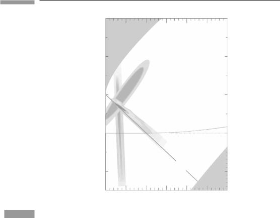
The variety of possible cosmological evolutions and the data are captured in the diagram in Fig. 12.4. The evidence is getting rather strong that the dark energy is present, and even dominant. That raises new, important questions. The deepest is, where in physics does this energy come from? We will mention below some of the speculations, but at present there is simply no good theory for it. In such a situation, better data might help. For example, astronomers could try to determine if the dark energy density really is constant in time (as it would be if it comes from a cosmological constant) or variable, which would indicate