

5 |
1.4 Spacetime diagrams |
The SI units contain many ‘derived’ units, such as joules and newtons, which are defined in terms of the basic three: m, s, kg. By converting from s to m these units simplify considerably: energy and momentum are measured in kg, acceleration in m−1, force in kg m−1, etc. Do the exercises on this. With practice, these units will seem as natural to you as they do to most modern theoretical physicists.
1.4 S p a ce t i m e d i a g ra m s
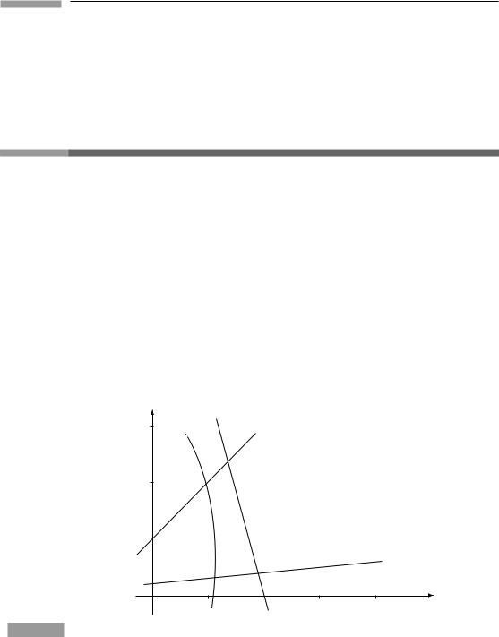
A very important part of learning the geometrical approach to SR is mastering the spacetime diagram. In the rest of this chapter we will derive SR from its postulates by using spacetime diagrams, because they provide a very powerful guide for threading our way among the many pitfalls SR presents to the beginner. Fig. 1.1 below shows a twodimensional slice of spacetime, the t − x plane, in which are illustrated the basic concepts. A single point in this space5 is a point of fixed x and fixed t, and is called an event. A line in the space gives a relation x = x(t), and so can represent the position of a particle at different times. This is called the particle’s world line. Its slope is related to its velocity,
slope = d t/dx = 1/v.
Notice that a light ray (photon) always travels on a 45◦ line in this diagram.
Figure 1.1
t
(m)
Accelerated
world line
World line of light, v = 1
World line of particle moving at speed |v| < 1
 An event
World |
line |
with |
velocity |
v>1 |
|
||||
|
|
|||
|
|
|
||
|
|
|
|
x (m)
A spacetime diagram in natural units.
5We use the word ‘space’ in a more general way than you may be used to. We do not mean a Euclidean space in which Euclidean distances are necessarily physically meaningful. Rather, we mean just that it is a set of points that is continuous (rather than discrete, as a lattice is). This is the first example of what we will define in Ch. 5
to be a ‘manifold’.

6 |
Special relativity |
We shall adopt the following notational conventions:
(1) |
Events will be denoted by cursive capitals, e.g. A, B, P. However, the letter O is |
|||
|
reserved to denote observers. |
|
|
|
(2) |
The coordinates will |
be |
called |
(t, x, y, z). Any quadruple of numbers like |
|
(5, −3, 2, 1016) denotes |
an |
event |
whose coordinates are t = 5, x = −3, y = 2, |
z = 1016. Thus, we always put t first. All coordinates are measured in meters.
(3)It is often convenient to refer to the coordinates (t, x, y, z) as a whole, or to each indifferently. That is why we give them the alternative names (x0, x1, x2, x3). These superscripts are not exponents, but just labels, called indices. Thus (x3)2 denotes the square of coordinate 3 (which is z), not the square of the cube of x. Generically, the coordinates x0, x1, x2, and x3 are referred to as xα . A Greek index (e.g. α, β, μ, ν) will be assumed to take a value from the set (0, 1, 2, 3). If α is not given a value, then xα is any of the four coordinates.
(4)There are occasions when we want to distinguish between t on the one hand and (x, y, z) on the other. We use Latin indices to refer to the spatial coordinates alone. Thus a Latin index (e.g. a, b, i, j, k, l) will be assumed to take a value from the set (1, 2, 3). If i is not given a value, then xi is any of the three spatial coordinates. Our
conventions on the use of Greek and Latin indices are by no means universally used by physicists. Some books reverse them, using Latin for {0, 1, 2, 3} and Greek for {1, 2, 3};
others use a, b, c, . . . for one set and i, j, k for the other. Students should always check the conventions used in the work they are reading.
1.5 Co n s t r u c t i o n o f t h e co o rd i n a t e s u s e d b y a n o t h e r o b s e r v e r
Since any observer is simply a coordinate system for spacetime, and since all observers look at the same events (the same spacetime), it should be possible to draw the coordinate lines of one observer on the spacetime diagram drawn by another observer. To do this we have to make use of the postulates of SR.
Suppose an observer O uses the coordinates t, x as above, and that another observer O¯ , with coordinates ¯t, x¯, is moving with velocity v in the x direction relative to O. Where do the coordinate axes for ¯t and x¯ go in the spacetime diagram of O?
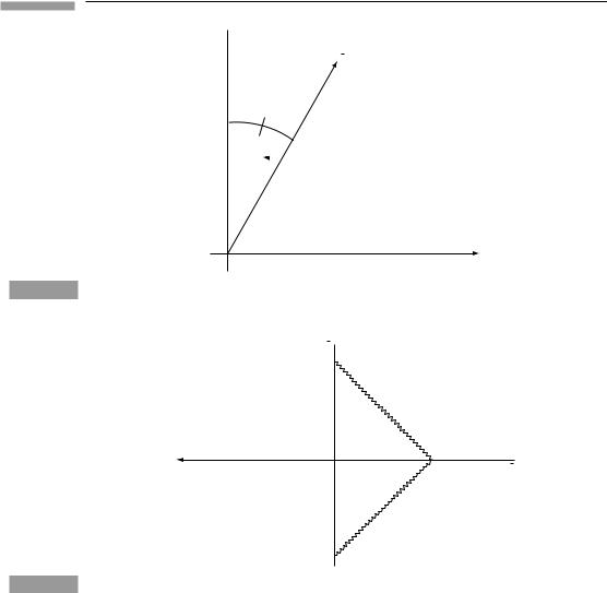
¯t axis: This is the locus of events at constant x¯ = 0 (and y¯ = z¯ = 0, too, but we shall ignore them here), which is the locus of the origin of O¯ ’s spatial coordinates. This is O¯ ’s world line, and it looks like that shown in Fig. 1.2.
x¯ axis: To locate this we make a construction designed to determine the locus of events at ¯t = 0, i.e. those that O¯ measures to be simultaneous with the event ¯t = x¯ = 0.
Consider the picture in O¯ ’s spacetime diagram, shown in Fig. 1.3. The events on the x¯ axis all have the following property: A light ray emitted at event E from x¯ = 0 at, say, time ¯t = −a will reach the x¯ axis at x¯ = a (we call this event P); if reflected, it will return to the point x¯ = 0 at ¯t = +a, called event R. The x¯ axis can be defined, therefore, as the locus of
7
Figure 1.2
Figure 1.3
1.5 Construction of the coordinates used by another observer
t 
t
 Tangent of this angle is υ
x
The time-axis of a frame whose velocity is v.
t a
a x
–a
Light reflected at a, as measured by O¯ .
events that reflect light rays in such a manner that they return to the ¯t axis at +a if they left it at −a, for any a. Now look at this in the spacetime diagram of O, Fig. 1.4.
We know where the ¯t axis lies, since we constructed it in Fig. 1.2. The events of emission and reception, ¯t = −a and ¯t = +a, are shown in Fig. 1.4. Since a is arbitrary, it does not matter where along the negative ¯t axis we place event E, so no assumption need yet be made about the calibration of the ¯t axis relative to the t axis. All that matters for the moment is that the event R on the ¯t axis must be as far from the origin as event E. Having drawn them in Fig. 1.4, we next draw in the same light beam as before, emitted from E, and traveling on a 45◦ line in this diagram. The reflected light beam must arrive at R, so it is the 45◦ line with negative slope through R. The intersection of these two light beams must be the event of reflection P. This establishes the location of P in our diagram. The line joining it with the origin – the dashed line – must be the x¯ axis: it does
8 |
Special relativity |
t
t
a
x
x
|
|
–a |
|
|
|
|
|
The reflection in Fig. 1.3, as measured . |
Figure 1.4 |
||
|
|
O |
t |
t |
|
t |
t |
|
φ |
|
φ |
|
||
|
|
|
|
||
|
|
x |
|
|
|
|
|
φ |
|
|
|
|
|
x |
|
φ |
x |
|
|
|
|
||
|
|
|
|
|
x |
(a) |
|
|
|
(b) |
|
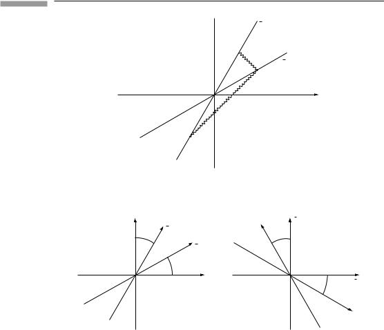
Figure 1.5 |
Spacetime diagrams of O (left) and O¯ (right). |
not coincide with the x axis. If you compare this diagram with the previous one, you will see why: in both diagrams light moves on a 45◦ line, while the t and ¯t axes change slope from one diagram to the other. This is the embodiment of the second fundamental postulate of SR: that the light beam in question has speed c = 1 (and hence slope = 1) with respect to every observer. When we apply this to these geometrical constructions we immediately find that the events simultaneous to O¯ (the line ¯t = 0, his x axis) are not simultaneous to O (are not parallel to the line t = 0, the x axis). This failure of simultaneity is inescapable.
The following diagrams (Fig. 1.5) represent the same physical situation. The one on the left is the spacetime diagram O, in which O¯ moves to the right. The one on the right is drawn from the point of view of O¯ , in which O moves to the left. The four angles are all equal to arc tan |v|, where |v| is the relative speed of O and O¯ .