UnEncrypted

Meta-epidemic model

Figure 1: Scheme of the model

2Model formulation

We consider two compartmentalized environments containing each individuals of a population, subject to a transmissible disease, so that they can be either susceptible or infected, Si and Ii, i = 1, 2, respectively.

We assume that mij is the susceptibles’ migration rate from environment j to environment i, with i, j = 1, 2. Similarly, let nij denote the migration rate of infected from environment j to environment i, with i, j = 1, 2. In principle they are di erent as migrations, entailing in general an e ort, are perhaps less possible for infected, that in view of the disease, are weaker individuals. We assume the disease to be recoverable, and that the recovery rate may be influenced by the environment. Thus let ν and η denote these rates. We also assume that ecological conditions in the two environments are in principle di erent, thereby a ecting the disease propagation and its recovery. Thus, the disease transmission rate in the first environment is γ while it is β in the second one. Overall, then, we have two copies of the classical SIS model linked via migrations. A schematic representation of the situation is graphically illustrated in Figure 1.

Using mass action incidence to model disease transmission, the model thus becomes

Marika Barengo, Isabella Iennaco, Ezio Venturino

Further, like in the classical epidemic models, [1], we make the assumption that the total population in the two enviroments has a constant value N, so that the recruitment rate of newborns matches the mortality rate, natural plus disease-related. Thus, S1 + I1 + S2 + I2 = N, and this is reflected by the fact that on summing the equations in (1), we find

2.1 Analysis of the equilibria

For the system (2) there are only two possible equilibria, in addition to the origin E(0) = (0, 0, 0), which is an equilibrium only if the total population vanishes, as consequence of

To find the components of the coexistence equilibrium, we sum the second and the third equilibrium equations thereby replacing the second one, and solve the third one to get the

where we set E ≡ −γ(M1 + M3), F ≡ 12 γ(M2 − M3), G ≡ 12 (γNM3 − n21 − ν), H ≡ 12 n12, A ≡ β(M0 + M2), B ≡ 12 β(M0 − M1), C ≡ 12 (n12 + η − βNM0) and D ≡ − 12 n21.

Equations (5) and (6) identify two conic sections, both through the origin and respectively intersecting the coordinate axes at the points (−2GE−1, 0) and (0, −2CA−1). The former conic for

In case n12 = m12 it becomes a parabola with axis x = − GE and vertex (−GE−1, G2(2EH)−1), with negative height there since EH = −n12γ(M1 + M3) < 0. The degenerate case

For n21 = m21 it becomes a parabola with axis y = −CA−1 and vertex (C2(2DA)−1, −CA−1). It also has negative height at the vertex in view of the fact that 2DA = −n21β(M0 +M2) < 0. The degenerate case is obtained if

Marika Barengo, Isabella Iennaco, Ezio Venturino

giving thus the two straight lines

y = − DB , x = − 2AB y. (12)

These conic sections will always intersect in the first quadrant, providing a feasible equilibrium if (4) is satisfied, but for the degenerate cases for which HF > 0 and DB > 0 (or equivalently F E < 0 and AB < 0). In the degenerate cases, we can explicitly write the equilibrium:

From the equilibria that we just found, we observe that it is not possible that the disease becomes a pandemic in the environment, i.e. it invades the whole population and the susceptibles totally disappear. This represents a good result from the epidemiological point of view.

2.2Stability

For the stability analysis we write the Jacobian J = (Jik), i, k = 1, 2, 3 of the system (2):

For the origin E(0), one eigenvalue can be immediately evaluated, −(m12 + m21) < 0, the remaining ones are the roots of a quadratic stemming from a suitable 2 × 2 submatrix

so that E(0) is always stable. Recall again, compare the discussion at the beginning of Section 2.1, that this means that the whole population is wiped out, including S1 which do not explicitly appear in the model. This result is not good from the environmental point of view, since the population disappears completely, but it should be expected. In fact, if the population drops it will never be able to recover as no such specific mechanisms are present in the model.

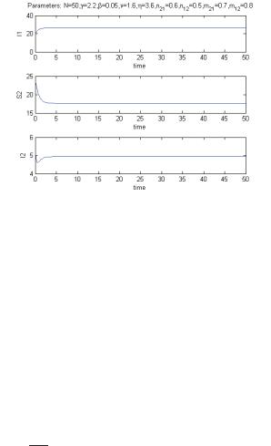
For the parameters N = 50, γ = 2.2, β = 0.05, ν = 1.6, η = 3.6, n21 = 0.6, n12 = 0.5, m21 = 0.7, m12 = 0.8, we find the coexistence equilibrium indeed at a stable state, see Figure 2.

3The case of migration only in one direction

We assume now that migration from patch 2 into patch 1 is not possible, m12 = n12 = 0,

Marika Barengo, Isabella Iennaco, Ezio Venturino

Figure 2: Coexistence at a stable state.

For E(0) ≡ E(0) = (0, 0, 0), the results of the stability analysis still hold, together with

For the coexistence equilibrium (2) in this case recall that M0 = 1, M2 = M3 = 0.

E

Thus S2 = N − I1 − I2 + mn2121 I1 > 0. The conic (5) becomes now just the pair of straight lines

Meta-epidemic model

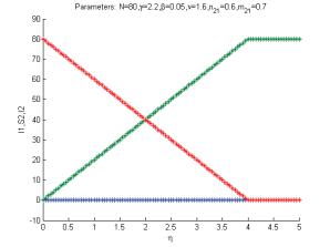
Figure 3: Transcritical bifurcation as function of the parameter η, for the case with the migrations from environment 2 to environment 1 forbidden.

Thus in this case the disease is eradicated and the whole healthy population settles only in patch 2.

the parameter values N = 80, γ = 2.2, β = 0.05, γ = 1.6, n21 = 0.6, m21 = 0.7.

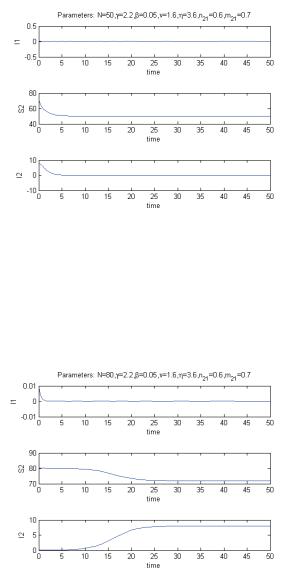
Thus if the ratio of disease recovery over the disease incidence in the second environment

is lower than the total population , see (18), then (1) is the only stable equilibrium, so

N E

that the disease is eradicated and the whole population settles in the second enviroment. This is shown in Figure 4 for the parameter values N = 50, γ = 2.2, β = 0.05, γ = 1.6, η = 3.6, n21 = 0.6, m21 = 0.7.

On the contrary, if the above condition is not satisfied, the disease becomes endemic and the whole population, susceptibles and infected, still settles in the second environment,

since in this case the equilibrium (3) becomes feasible, (17) and is stable. See Figure 5

E

for a graphical description with the parameter values N = 80, γ = 2.2, β = 0.05, γ = 1.6, η = 3.6, n21 = 0.6, m21 = 0.7.

Marika Barengo, Isabella Iennaco, Ezio Venturino

Figure 4: Equilibrium (1) for the case with the migrations from environment 2 to environ-

E

ment 1 forbidden.

Figure 5: Equilibrium (3) for the case with the migrations from environment 2 to environ-

E

ment 1 forbidden.

Meta-epidemic model

4Infected do not migrate

In this situation, let us denote the equilibria as E(k), for k = 0, . . . , 4. Here n12 = n21 = 0, so that M1 = M2 = 0. Again at the origin the conclusions of the original system (2) still hold. In particular we then find E(1) ≡ E(1), E(3) with nonzero components

For the coexistence equilibrium E(2) we have the following considerations. The two conic sections become now both degenerate: in the first case we have I1 = 0 and I2 = −I1 − (ν +γM0N)(γM3)−1, for the second one instead I2 = 0 and I2 = −N−1I1 +1−η(βNM0)−1. No intersections of these lines in the interior of the first quadrant are therefore possible, hence no coexistence equilibrium exists in this case.

The eigenvalues of the Jacobian at E(1) are −m12 − m21 < 0 and the pair βNM0 − η,

Marika Barengo, Isabella Iennaco, Ezio Venturino

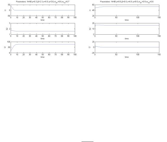
Figure 6: Left: stability of the equilibrium E(3). Right: stability of the equilibrium E(4).

But the inequalities (24) hold unconditionally when the equilibrium is feasible, in view of (20), so that stability reduces to just condition (23).

Again, there is a transcritical bifurcation when E(3) and E(4) exchange their stability. This is influenced by the value of the parameter

ρ≡ βνM0 γηM3

being smaller or larger than 1. Further, when E(1) is stable, it is the only feasible equilibrium, while when either E(3) or E(4) are feasible, E(1) is always infeasible.

Thus in this case the disease gets eradicated from the ecosystem, if the system settles to equilibrium E(1). Else at E(3) it is eradicated only in environment 1, see Figure 6 left, or finally at E(4) it is eradicated only in environment 2, see Figure 6 right. No other possibilities exist, when the ecosystem thrives.

5Conclusions

We now discuss briefly some consequences that can be drawn from the above analyses. Recall that all these systems are fragile, in the sense that the whole population can vanish,