UnEncrypted

Richard K. Bowles, Cletus C. Asuquo

0.3

Q s

0.2

0.1

Qb

Figure 2: Qs as a function of Qb for the di erent solid structures.

influence the probabilities of seeing the di erent structures in condensed phases, particularly in the low barrier regime.

Acknowledgements

We thank NSERC for financial support.

References

[1]D. J. Wales, Energy Landscapes, With Applications to Clusters, Biomolecules and Glasses, Cambridge University Press, Cambridge, 2003.

[2]Y. H. Xiang, L. J. Cheng, W. S. Cai and X. G. Shao, Structural distribution of LennardJones clusters containing 562 to 1000 atoms, J. Chem. Phys. 108 (2004) 9516-9520.

Freezing in Gold Nanoclusters

[3]I. Saika-Voivod, L. Poon and R. K. Bowles, The role of fcc tetrahedral subunits in the phase behavior of medium sized Lennard-Jones clusters, J. Chem. Phys. 133 (2010) 074503.

[4]Y. G. Chushak and L. S. Bartell, Melting and freezing of gold nanoclusters, J. Phys. Chem. B (2001) 105 11605-11614.

[5]P. J. Steinhardt, D. R. Nelson and M. Ronchentti, Bond-orientational order in liquids and glasses, Phys. Rev. B (1983) 28 784-805.

[6]Y. Wang, S. Teitel and C. Dellago, Melting of icosahedral gold nanoclusters from molecular dynamics simulations, J. Chem. Phys. (2005) 122, 214722.

[7]S. C. Hendy and J. P. K. Doye, Surface-reconstructed icosahedral structures for lead clusters Phys. Rev. B. (2002) 66 235402.

[8]H.-S. Nam, N. M. Hwang, B. D. Yu and J.-K. Yoon, Formation of an icosahedral structure during the freezing of gold nanoclusters: Surface-induced mechanism, Phys. Rev. Lett. (2002) 89 275502.

[9]E. Mendez-Villuendas and R. K. Bowles, Surface nucleation in the freezing of gold nanoparticles, Phys. Rev. Lett. (2007) 98 185503.

[10]D. P. Sanders, H. Larralde and F. Leyvraz, Competitive nucleation and the Ostwald rule in a generalized Potts model with multiple metastable phases, Phys. Rev. B (2002)

75 132101.

Proceedings of the 12th International Conference on Computational and Mathematical Methods

in Science and Engineering, CMMSE 2012 July, 2-5, 2012.

Cluster Model of Total - Connected Flow with Local Information

Alexander P. Buslaev1 and Marina V. Yashina2

1 Department of Mathematics, Moscow State Automobile and Road Tech. University

2 Department of Mathematical Cybernetics and IT , Moscow Technical University of

Communications and Informatics

emails: apal2006@yandex.ru, yash-marina@yandex.ru

Abstract

We introduce some model of a flow. The flow is represented as a sequence of synchronized packets of particles, which move with the velocity depended on the flow density and interact by given laws.

Some quality properties of corresponded system of ordinary di erential equations are developed.

Key words:

System of nonlinear di erential equations, theory of tra c flow, following-the-leader model, cluster model of particles movement

MSC 2000: AMS codes 74H05, 91F99

1Introduction

One of the basic models of tra c flow, follow-the-leader model, [1] - [5], [12], can be reduced to the study of di erential equations of the following type

We call the flow satisfying the conditions (1)-(2) as total - connected flow.

Steady state, x˙ n(t) ≡ Cn, n = 1, ..., is equivalent to x˙ n+1(t) ≡ x˙ n(t), i.e. xn+1 − xn ≡ C are uniformly located elements of the flow.

Hence, the steady state of the chain x1 < x2 < ... < xn is equivalent to a uniformly moving cluster with the velocity v = f −1(C) and the density ρ = C−1.

Cluster Model of Total - Connected Flow with Local Information

2Connected flow of stationary clusters

We assume the flow support consists of clusters. The cluster moves along a straight line at velocity

The function g(ρ) is called a state function. The simplest type of a state function is linear function 0 ≤ ρ ≤ ρmax, g(0) = vmax, g(ρmax) = 0. For simplicity, we assume

vmax = ρmax = 1.

Strategy of a total-connected flow needs the velocity regime of the follower to be adjusted to the velocity regime of the leader. That restricts the separation of flow to independent parts in the sense discussed below.

Neighboring clusters, i.e. leader and follower, interact with each other by information transfer inside the follower.

If only the leading edge of the follow cluster has the information on the approaching contact with leader, then this part of follower begins to transform itself to adapt to speed mode of the leader.

We refer to such a model as a cluster model of flow with local information.

3Interation of clusters local information

We consider two available scenarios.

3.1The slow cluster follows the fast leader

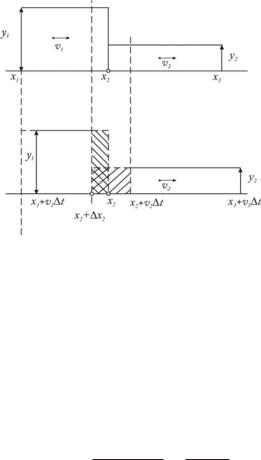
As the leading cluster has great velocity, the rising edge of the follower is transforming in the tail of leader with preservation of total mass of particles.

We derive di erential equations for interaction between these two clusters.

Suppose that at time t the base of the left (following) cluster, i.e. cluster, which is behind, is the segment (x1, x2), and its height, i.e. flow density on the segment (x1, x2), equals to y1, Fig.1.

The base of the cluster, which is moving ahead, is interval (x2, x3), having a height of

coincides with the left edge of the right cluster moves with a speed that satisfies the condition that sum of the areas of rectangles remains constant.

Alexander P. Buslaev, Marina V. Yashina

Figure 1: The slow cluster follows the fast cluster

Let x2 + x2 be a coordinate of the point on the x-axis corresponding to the boundary at time t + t.

We have for the case of movement of the slow cluster behind the fast cluster (Fig. 1):

(x2 + v2 t − x2 − x2) y2 = ((x2 − x1) − (x2 + x2 − x1 − v1 t))y1,(v2 t − x2)y2 = (− x2 + v1 t)y1,

(v2y2 − v1y1)Δt = x2(y2 − y1),

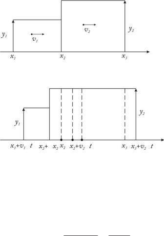
3.2The fast cluster follows the slow leader

We now assume that the slow cluster is moving ahead of the fast cluster (Fig. 2). Rising edge of the faster follower cluster is transformed into the stern of a slow cluster. Then the boundary of the clusters contact varies taking into account the conservation law of particles.

Hence (Fig.2)

(x2 + v2 t − x2 − x2)y2 = ((x2 − x1) − (x2 + x2 − x1 − v1 t))y1,

Cluster Model of Total - Connected Flow with Local Information

Figure 2: The fast cluster follows the slow cluster

4Cluster model on a ring

Assume a circle is divided into n segments

0 ≤ x01 < x02 < . . . < x0n < 1 < x0n+1 = x1 + 1

Alexander P. Buslaev, Marina V. Yashina

At each segment [x0i , x0i+1] there is defined a density yi, 1 ≤ i ≤ n. Velocity of i−th cluster is determined by the function vi = g(yi). In accordance with Section 3, we have the

following dynamical system

Research of solutions of the system (6) allows to determine quantitative properties of the model. For simplicity, we consider

(x˙ i+1 − x˙ i) = (xi+1 − xi)˙ = −(yi+1 − yi−1).

Lemma 2. Suppose that maxi(yi+1 − yi) > 0, in particular, when number n is even, yi = Const. Then for 1 ≤ i ≤ n,

the model is described by the system (6) up to the numbering and the number of variables k = k(n) < n.

Proof. It follows from (9).

We call a stationary k-th orbit any set {y1, ...yn}, such that the system (6) has a stationary solution at n = k.

Lemma 3. Let y = (y1, ...yn) be stationary n−th orbit

a)n is even, yi−1 = yi+1 = ... = y, yi = yi+2 = ... = 1 − y, y = 0.5;

b)n is arbitrary, y = 0.5(1, ...1).

Proof.

If yi+1 + yi = 1, i = 1, ...n, then all yi with even indexes and all yi with odd indexes are the same.

Cluster Model of Total - Connected Flow with Local Information

We call a dynamic k−th orbit any set {y1, ...yk }, such that (xi+1 − xi)(t) ≡ Ci, i = 1, ..., k.

In particular, when k = 2 equalities (10) are trivial.

Theorem. If {yi} are di erent, then system (6) , in general position, is reduced to a dynamic 2 - orbit at finite time.

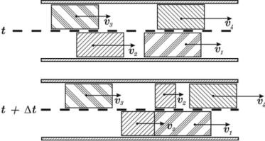
5Cluster model of total connected multilane movement

For simplicity we suppose the lane number is m = 2. If the fast cluster is catching up to the slow cluster, then, under the condition of a free lane, fast cluster flows into the adjacent lane at the contact level, keeping its velocity and density.

If the adjacent lane is busy, the change of the fast cluster into a slow performs by the scenario described in the preceding paragraphs to the moment when the adjacent lane would be free.

Figure 3: Two lanes cluster flow

The main problem is to describe the dynamics of two-lane cluster model and research the existence problem for a stationary state. Obviously, the number of values of densities {yi} can not increase. However, at the lane changing, the division of a cluster can occur, so the total number of clusters can increase.

Alexander P. Buslaev, Marina V. Yashina

6Conclusions

The study approach combines the collective and individual characteristics of the behavior of elementary flow components, as result of which the movement reduces to interaction of clusters, that are conditionally - stationary in the sense of hydrodynamic models, [6]. On the other, clusters can be considered as particals with behaviour described by probabilistic approach, [7 - 9].

The resulting mathematical problems are independent interest, in spite of the fact that computational algorithms are created and tested, which results also can be discussed.

Acknowledgements

This work has been supported by by Ministry of Education and Science of the Russian Federation, project No.14.740.11.0397, and grant of RFBR No.11-01-12140-ofi.

References

[1]R. B. Morisson The Tra c Flow Analogy to Compressible Fluid Flow, Advanced Res. Eng. Bull., 1964.

[2]Hiroshi Inose, Takashi Hamada. Road Tra c Control. University of Tokyo Press. 1975

[3]R. W. Rothery Car Following Models in Tra c Flow Theory, Transportation research board, ed. Gartner N , Special report, 165 (1992) 4.1 – 4.42.

[4]Pipes L.A. An operational Analysis of Tra c Dynamics, Journal of Applied Physics,

24 (1953) 271–281.

[5]Buslaev A.P., Gasnikov A.V., Yashina M.V. Mathematical Problems of Tra c Flow Theory. Proceed. of the 2010 International Conference on Computational and Mathematical Methods in Science and Engineering, ed J.Vigo Aguar, Almeria, Spain, 26-30.06.2010, v.1, (2010) p.307-313

[6]Lighthill M.L., Whitham G.B. On kinematic waves. A theory of tra c flow on long crowed roads. Proceedings of the Royal Society of London, Piccadilly, London, (1955) A229 (1170) 317–345.

[7]Nagel K., Schreckenberg M. A cellurar automation model for freeway tra c. J. Physique. France, 2 (1992), 2221–2229.

Cluster Model of Total - Connected Flow with Local Information

[8]C.F. Daganzo. The cell transmission model: A dynamic representation of highway tra c consistent with the hydrodynamic theory. Transp.Res. B. V.28, 4 (1994) 269–287.

[9]C.F. Daganzo. The cell transmission model, Part II: Network tra c. Transp.Res. B. V.29, 2 (1995) 79–93.

[10]Nazarov A.I. On stability of stationary modes in a system of nonlinear ODE arising in modeling of tra c flows. Vestnik SPbGU, S.1, 3 (2006) (In Russian)

[11]A.P. Buslaev, A.V. Provorov, M.V. Yashina. Current approaches to the study of connected flow of particles with motivation. T-Comm. J. Telecommunications and Transport, 2 (2011) 61–62 (In Russian)

[12]A.P. Buslaev, A.V. Gasnikov, M.V.Yashina. Selected Mathematical Problems of Tra c Flow Theory. International Journal of Computer Mathematics. Volume 89, 3 , Special Issue: Topics of Contemporary Computational Mathematics. Section B. (2012) 409–432 DOI:10.1080/00207160.2011.611241