UnEncrypted

Proceedings of the 12th International Conference on Computational and Mathematical Methods in Science and Engineering, CMMSE 2012 July, 2-5, 2012.

Increasing the exactness of spline quasi-interpolants

D. Barrera1, A. Guessab2, M. J. Ib´a˜nez1 and O. Nouisser3

1 Departamento de Matem´atica Aplicada, Universidad de Granada

2 Laboratoire de Math´ematiques Appliqu´ees, Universit´ de Pau et des Pays de l’Adour

3 D´epartement de Math´ematiques et Informatique, Universit´ Cadi-Ayyad

emails: dbarrera@ugr.es, allal.guessab@univ-pau.fr, mibanez@ugr.es, otheman.nouisser@yahoo.fr

Abstract

Given a spline discrete quasi-interpolation operator Qd, which is exact on the space Pm of polynomials of total degree at most m, we propose a general method to determine a new di erential quasi-interpolation operator QDr which is exact on Pm+r. QDr uses the values of the function to be approximated at the points involved in the linear functional defining Qd as well as the partial derivatives up to the order r at the same points. From this result, we then construct and study a first order di erential quasi-interpolant based on the C1 B-spline on the equilateral triangulation with an hexagonal support.

Key words: B-splines, Box splines, Di erential Quasi-interpolants, Discrete quasiinterpolants, Optimal approximation order

1Introduction

Quasi-interpolation based on a B-spline is a general approach for e ciently constructing approximants, with low computational cost. Its e ectiveness is particularly due to its small support, to achieve local control via suitable spline coe cients in the space spanned by the translates of the B-spline.

In the recent paper [2], it is shown how to modify a given linear operator such that the resulting operator reproduces polynomials to the highest possible degree, and such that the approximation order is the best possible.

As a main application of this tool, new spline quasi-interpolation operators are derived, based on a uniform type-1 triangulation τ approximating regularly distributed data.

Increasing the exactness of spline quasi-interpolants

2Notations

degree included in the space S (M) spanned by translates of M. We will assume that

P (M) = Pm for some positive integer m.

For a real valued function f and k N, we say f Ck R2 if f is k times continuously

di erentiable in the following sense: the directional derivatives of order l, l = 0, . . . , k, at x R2 along the direction y R2 defined as

Dl f (x) = dll f (x + ty)|t=0 y dt

exist and depend continuously on x. When the directional derivative exists for y, it may be extended to multiples by defining

3Modified di erential bivariate spline quasi-interpolants

We are interested in the dQIO Qd based on the B-spline M Skl (τ) given by the expression

where λ is the linear functional defined as λf := j J cj f (−Aj ), for a finite subset J Z2 and c := (cj )j J R#J , with #J denoting the cardinality of J (cf. [1, p. 63]). Qd is a linear map into S (M) which is local and bounded, and we shall construct Qd to reproduce

Pm.

We will assume that the free parameters cj , which define the functional λ, are given in such a way that Qd is exact on Pm. So, Qd achieves the order of approximation m + 1.

D. Barrera, A. Guessab, M. J. Iba´nez,˜ O. Nouisser

j J

If in (2) we replace f (Ai) by its Taylor polynomial approximation of degree r at Ai, then the resulting operator

reproduces polynomials up to degree m + r. This result is a consequence of the following integral representation of the error for the quasi-interpolants QDr .

where Kmr (t) := (−1)m tm(1−t)r .

(m+r)!

As another immediate corollary of Theorem 1, we obtain the following error estimate.

Increasing the exactness of spline quasi-interpolants

We may estimate the approximation error as a function of the free parameters cj , when the function to be approximate is su ciently regular. Indeed, by (3), the sum in the function R (x) involved in the error estimate established in equations (7)-(8) may be written in terms

=: F (c, x)

One possible strategy would be to select the free parameters cj , in the starting operator Qd, in such a way to minimize the upper bound function F (c, x) subject to equality constraints on cj , yielding the exactness of Qd on Pm. However, in order to obtain a much simpler minimization problem, we suggest a formulation with an upper bound F (c) of F (c, x), depending only on c.

Due to the interesting properties of C1 quartic splines on type-1 triangulations, we will solve this kind of problem starting from the C1 cubic B-spline defined on the equilateral triangulation of the real plane, under specific imposed conditions on the sequence c. We will give a detailed treatment including an explicit error bound estimation for the corresponding operator, which are especially useful in practice.

References

[1]C. de Boor, K. H¨ollig and S. Riemenschneider, Box splines, Springer-Verlag, New York.

[2]A. Guessab, O. Nouisser and G. Schmeisser, Multivariate approximation by a combination of modified Taylor polynomials, J. Comput. Appl. Math. 196 (2006), 162–179.

Proceedings of the 12th International Conference on Computational and Mathematical Methods in Science and Engineering, CMMSE 2012 July, 2-5, 2012.

A new more consistent Reynolds model for piezoviscous hydrodynamic lubrication problems in line contact devices

Guy Bayada1, Bego˜na Cid2, Guillermo Garc´ıa2 and Carlos V´azquez3

1 ICJ UMR CNRS 5208, INSA de Lyon

2 Department of Applied Mathematics II, University of Vigo

3 Department of Applied Mathematics, University of A Coru˜na

emails: Guy.Bayada@insa-lyon.fr, bego@dma.uvigo.es, guille@dma.uvigo.es, carlosv@udc.es

Abstract

Hydrodynamic lubrication problems in piezoviscous regime are usually modeled by the classical Reynolds equation combined with a suitable law for the pressure– dependence of viscosity. By taking into account the pressure–viscosity dependence in the Stokes equation and to derive the Reynolds equation in the thin film limit, a new model has been proposed by Rajagopal & Szeri [5]. However, in [5] some additional simplifications are assumed. In the present work, avoiding these simplifications, from a Stokes equation in piezoviscous regime we deduce a new Reynolds model for line contact lubrication problems, in which the cavitation phenomenon is also taken into account. Thus, the new complete model consists of a nonlinear free boundary problem associated to the proposed new Reynolds equation.

Moreover, the classical model, Szeri’s one and the here proposed one are simulated through the development of some numerical algorithms involving upwind schemes, finite elements method, duality type numerical strategies and fixed point techniques. Finally, several numerical tests are performed to carry out a comparative analysis among the di erent models.

Key words: Hydrodynamic lubrication, Reynolds equation, piezoviscosity, cavitation phenomenon, free boundary

A more consistent Reynolds model

1Introduction

In the mechanical and mathematical literature concerning the models for piezoviscous hydrodynamic lubrication problems, di erent classical devices have been considered, such as journal–bearings, rolling–bearings, rolling–ball–bearings,. . . In all of these situations, the behavior of the lubricant pressure in the thin film setting has been classically modeled by the Reynolds equation, in which the pressure–dependence of viscosity is usually introduced a posteriori by some expression, such as, for example, the Barus law:

where μ, μ0, p and α denote the viscosity, the zero pressure viscosity, the pressure and the piezoviscosity coe cient. In this procedure, the thin film limit from Stokes equation to Reynolds one is obtained regardless of the pressure–viscosity dependence. Moreover, the cavitation phenomenon can be incorporated through Reynolds model or Elrod–Adams one (see [1], for instance). However, by assuming that the viscosity depends on pressure in Stokes equation according to Barus law, in [5] a more careful derivation of the limit Reynolds equation is carried out. More precisely, after some simplifying assumptions the

where h, (u, v) and (s, 0) denote the gap between surfaces, the velocity field in the thin film and the velocity field at the lower surface, assuming that the upper surface is fixed. Next, by approximating ∂ u/∂ x by d uav/d x where uav is an average velocity, they introduce the

2An alternative model for piezoviscous lubrication

In this work, mainly a more rigorous model avoiding the simplification considered in [5] is proposed. Indeed, a new equation for the case of a line contact with Reynolds model for cavitation is obtained. The proposed methodology to deduce a new family of models is based on a fixed point technique to solve the equations (2)-(3), starting from an initial velocity u0(x, y) which vanishes at the upper surface and is equal to (s, 0) at the lower one, satisfying the flux condition # h

u0(x, y) dy = Q. (5)

0

It is possible to use a fixed point technique just by replacing u0 in the second equation to obtain v0, next obtaining a new u1 in order to build a new Reynolds equation, and so on. In this way, each fixed point iteration provides a new model, however it does not seem possible to obtain a generic procedure and the complexity of the expressions involved is increasing. So the first iteration equation (7) is the model we consider here.

In order to compare the results with those of [5], we introduce the angular coordinate, t, by the change x = R sin(t), t [−π/2, π/2], where R is the radius of the cylinder. We define the film thickness by

and we introduce the following non-dimensional terms:

Furthermore, we consider the Reynolds model for cavitation (see [1], for example) and we obtain the following dimensionless formulation of the problem: find p, such that

being Ω+ = {t Ω/ p(t) > 0} and Ω0 = {t Ω/ p(t) = 0}. Moreover,

where t2 is the unknown free boundary and h0 denotes the minimum of the dimensionless gap. This model includes the isoviscous case (α = β = 0) and the classical piezoviscous

A more consistent Reynolds model

model (α = 0, β = 0). The Rajagopal & Szeri model may be written in a similar way but with a slightly di erent expression of G(t).

Note that problem (8)–(11) admits a formulation in terms of variational inequalities and their numerical solutions may be obtained by the combination of finite element techniques with classical projection methods or the more complex duality type algorithm ([2]). The application of these techniques to classical piezoviscous formulations can be found in [3] and [4], for example.

Another alternative is to restart from the modified Reynolds equation, to integrate it

In order to compute p and t2 we propose an iterative numerical scheme combining the ode15s integrator of MATLAB to solve (13)–(14) in [−π/2, t2], for each value of t2, with a regula falsi algorithm to search the final value of t2 (0, π/2), such that p(t2) = 0.

Note that the corresponding first order ODE version for isoviscous, classical piezoviscous and Rajagopal–Szeri models can be obtained in an analogous way and solved with the same numerical methods.

So far, we propose two alternatives for the numerical simulation: the use of a first order ode solver and the use of a characteristics finite elements method combined with a duality method to solve the free boundary problem associated to the second order elliptic equation.

3Numerical tests

In order to assess the relevance of both new more rigorous models for the piezoviscous case, several numerical tests have been carried out. The first impression is that the maximum

Bayada, Cid, Garc´ıa, Vazquez´

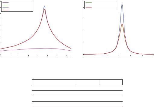
values of pressure are slightly di erent but the variation of the maximum values of viscosity are higher. In general, the solution of our alternative model appears to be closer to the classical solution than the one proposed in [5], as illustrated by Figure 1 and Table 1.

Table 1: Maximum dimensionless pressure for di erent models with first order EDO solver (ODE-R) and second order variational inequality solver (IV-R-BM)

A first conclusion is that the problem has a large gradient near the maximum pressure region so that is di cult to capture the almost “spike” qualitative behavior of the solution in all models. The here proposed one seems to be closer to the classical piezoviscous solution that the one proposed by Rajagopal and Szeri. In this sense, we have proposed a rigorous methodology to include piezoviscosity previously to the limit procedures followed for obtaining Reynolds model from Stokes one that overcomes the simplifications in [5]. Furthermore, it seems that the numerical results obtained for this new model in the regime we have considered result to be close to the ones obtained by the classical model mainly used in mechanical and mathematical literature.

Now we are trying to extend the use of the alternative model to the case in which Elrod– Adams model for cavitation is used, as it results more realistic when cavitation phenomenon

A more consistent Reynolds model

appears in the convergent region (starvation phenomenon).

Acknowledgements

This work has been partially supported by the MEC Research Project (MTM2010-21135- C02).

References

[1]G. Bayada and M. Chambat, Sur quelques mod´elisations de la zone de cavitation en lubrification hydrodynamique, J. of Theor. and Appl. Mech. 5(5) (1986) 703–729.

[2]A. Bermudez´ and C. Moreno, Duality methods for solving variational inequalities, Comp. Math. with Appl. 7 (1981) 43–58.

[3]N. Calvo, J. Durany and C. Vazquez´ , Comparaci´on de algoritmos num´ericos en problemas de lubricaci´on hidrodin´amica con cavitaci´on en dimensi´on uno, Rev. Int. Met. Num. Calc. Dis. Ing. 13, 2 (1997) 185–209.

[4]J. Durany, G. Garc´ıa and C. Vazquez´ , Numerical computation of free boundary problems in elastohydrodynamic lubrication, Appl. Math. Modelling 20 (1996) 104–113.

[5]K. R. Rajagopal and A. Z. Szeri, On an inconsistency in the derivation of the equations of elastohydrodynamic lubrication, Proc. R. Soc. Lond. A 459 (2003) 2771– 2786.

[6]O. Reynolds, On the theory of lubrication and its application to the Tower’s experiments, Phil Trans. R. Soc. Lond. 177 (1886) 159–209.

[7]A. Z. Szeri, Fluid film lubrication:theory and design, Cambridge University Press, 1998.