Lecture 4

Present (or Discounted) Value, Risk and Return

1. Present (or Discounted) Value

2. Risk and Return

3. Using probability distributions to measure

4. Expected Return and Standard Deviation

5. Risk and return at portfolio context

6. Risk diversification

Research work:

1. The main financial indicators of Ukraine and Crimea development for the last 5 years (sources!!!)

2. Financial problems of tourism in Crimea

Present (or Discounted) Value (приведенная [текущая, дисконтированная] стоимость [ценность] (сумма ожидаемого в будущем дохода или платежа, дисконтированная на основе той или иной процентной ставки). We all realize that a dollar today is worth more than a dollar to be received one, two, or three years from now. Calculating the present value of future cash flows allows us to place all cash flows on a current footing so that comparisons can be made in terms of today's dollars.

An understanding of the present value concept should enable us to answer a question that was posed earlier: which should you prefer—$1,000 today or $2,000 ten years from today? Assume that both sums are completely certain and your opportunity cost (альтернативная стоимость, цена возможности (стоимость сделанного выбора; эквивалентна выгоде, которую можно было бы получить в случае принятия наилучшего из отвергнутых вариантов) of funds is 8 % per annum (i.e., you could borrow or lend at 8 %). The present worth (текущая стоим) of $1,000 received today is easy—it is worth (стоим) $1,000. However, what is $2,000 received at the end of 10 years worth to you today? We might begin by asking what amount (today) would grow to be $2,000 at the end of 10 years at 8 percent compound interest. This amount is called the present value of $2,000 payable in 10 years, discounted at 8 percent. In present value it rate (capital- problems such as this, the interest rate is also known as the discount rate (or capital rate). Finding the present value (or discounting) is simply the reverse of compounding (начисление сложного процента (расчет будущей стоимости денежных потоков; процесс обратный дисконтированию)).

Therefore, let's first retrieve: FV_n = P₀(1 + i)ⁿ (1)

Rearranging terms, we solve for present value:

PV₀ = P₀=FVn/(1+i)^{n =}FVn*[1/(1 + i)ⁿ] (2)

Note that the term [1/(1 + i)ⁿ is simply reciprocal (обратный) of the future value interest factor at i% for n period (FVIFi,n). This reciprocal has own name -the present value interest factor at i% for n periods (PVIFi,n (коэф приведения

PV_o= FV_n(PVIF_i,n) (3)

TABLE 1

Present value interest factor of $1 at i% for n periods (PVIF_i,n)

(PVIFin)=1/(1 + i)n
PERIOD (n)		INTEREST RATE (i)
	1%		3%	5%	8%	10%	15%
1	0.990		0..971	0..952	0.926	0.909	0.870
2	0.980		0..943	0..907	0.857	0.826	0.756
3	0. 971		0..915	0.864	0.794	0.751	0.658
4	0.961		0..888	0..823	0.735	0.683	0..572
5	0.951		0..863	0.784	0.681	0.621	0.497
6	0.942		0..837	0.746	0.630	0.564	0.432
7	0.933		0..813	0.711	0.583	0.513	0..376
8	0.923		0.789	0.677	0.540	0.467	0..327
9	0.914		0.766	0.645	0.500	0.424	0..284
10	0.905		0.744	0.614	0.463	0.386	0..247

A present value table containing PVIF's for a wide range of interest rates and time periods relieves us of making the calculations. Table 1 is an abbreviated version of one such table. We can now make use the last formula and Table 1 to solve for the present value of $2,000 to be received at the end of 10 years, discounted at 8 percent. In Table 1, the intersection of the 8% column with the 10-years period row pinpoints PVIF _8%10—0.463. This tells us that $1 received 10 years from now is worth roughly 46 cents to us today. Armed with this information, we get

PV₀ = FV₁₀(PVIF _{8% 10})= $2,000(0.463) = $926

Finally, if we compare this present value amount ($926) to the promise of $1,000 to be received today, we should prefer to take the $1,000. In present value terms we would be better off by $74 ($1,000 - $926).

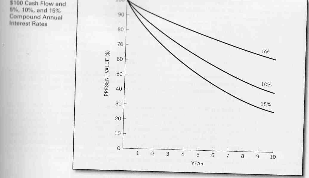
Discounting future cash flows turns out to be very much like the process of handicapping (уравновешивать условия, затруднять). That is, we put future cash flows at a mathematically determined disadvantage relative to current dollars. For example, in the problem just addressed, every future dollar was handicapped to such an extent that each was worth only about 46 cents. The greater the disadvantage assigned (присвоенный, ассигнованный) to a future cash flow, the smaller the corresponding present value interest factor (PVIF). Figure 1 illustrates how both time and discount rate combine to affect present value; the present value of $100 received from 1 to 10 years in the future is graphed for discount rates of 5,10, and 15 percent. The graph shows that the present value of $100 decreases by a decreasing rate the further in the future that it is to be received. The greater the interest rate, of course, the lower the present value but also the more pronounced the curve. At a 15 percent discount rate, $100 to be received 10 years hence is worth only $24.70 today—or roughly 25 cents on the (future) dollar.

Return

The return from holding an investment over some period—say, a year—is simply any cash payments received due to ownership, plus the change in market price, divided by the beginning price. You might, for example, buy for $100 a security that would pay $7 in cash to you and be worth $106 one year later. The return would be ($7 + $6)/$100 = 13%. Thus, return comes to you from two sources: income plus any price appreciation (or loss in price).

For common stock we can define one-period return as

R= [D_t+(P_t-P_t-1) ]/ P_t-1 (4)

where R is the actual (expected) return when t refers to a particular time period in the past (future);

D_t is the cash dividend at the end of time period t;

P_t is the stock's price at time period t; and

P_t-1 is the stock's price at time period t -1.

Notice that this formula can be used to determine both actual one-period returns (when based on his topical figures) as well as expected one-period returns (when based on future expected dividends and prices). Also note that the term in parentheses in the numerator of Eq. (5-1) represents the capital gain or loss during the period.

Risk

For example, you buy a share of common stock in any company and hold it for one year. The cash dividend that you anticipate receiving may or may not materialize as expected. And, what is more, the year-end price of the stock might be much lower than expected—maybe even less than you started with. Thus, your actual return on this investment may differ substantially from your expected return. If we define risk as the variability of returns from those that are expected, the T-bill would be a risk-free security while the common stock would be a risky security. The greater the variability, the riskier the security is said to be.

Using probability distributions to measure risk

As we have just noted, for all except risk-free securities the return we expect may be different from the return we receive. For risky securities, the actual rate of return can be viewed as a random variable (случайная величина) subject to a probability distribution (распределение вероятностей). Suppose, for example, that an investor believed that the possible one-year returns from investing in a particular common stock were as shown in the shaded section of Table 1, which represents the probability distribution of one-year returns. This probability distribution can be summarized in terms of two parameters of the distribution: (1) the expected return and (2) the standard deviation.

Expected Return and Standard Deviation ( среднеквадратичное отклонение -мера (оценка) риска для инвестиций, приносящих случайный доход; чем больше величина стандартного отклонения, тем выше риск)

The expected return (ожидаемый доход), R_e, is

R_e =Σ (Ri)(Pi) (5)

where Ri is the return for the i^th possibility, Pi- is the probability of that return occurring, and n is the total number of possibilities. Thus, the expected return is simply a weighted average (средневзвешенная) of the possible returns, with the weights being the probabilities of occurrence (случай). For the distribution of possible returns shown in Table 1, the expected return is shown to be 9 %.

TABLE 1. Illustration of the use of probability distribution of possible one year returns to calculate expected return and standard deviation

Possible return Ri	Probability of occurrence Pi	Expected return calculation Re	Variance calculation σ2
		(Ri)(Pi)	(Ri-Re)2(Pi)
-0.1	0.05	-0.005	(-0.1-0.09)2*0.05
-0.02	0.1	-0.002	(-0.02-0.09)2*0.1
0.04	0.2	0.008	(0.04-0.09)2*0.2
0.09	0.3	0.027	(0.09-0.09)2*0.03
0.14	0.2	0.028	(0.14-0.09)2*0.2
0.2	0.1	0.02	(0.0-0.09)2*0.1
0.28	0.05	0.014	(0.28-0.09)2*0.05
	Σ=1.00	Σ=0.09=Re	Σ=0.00703= σ2
			Standard deviation = (0.00703)0.5=0.0838= σ

To complete the two-parameter description of our return distribution, we need a measure of the dispersion (дисперсия, разброс), or variability (вариабельность, изменчивость), around our expected return. The conventional measure of dispersion is the standard deviation. The greater the standard deviation of returns, the greater the variability of returns, and the greater the risk of the investment. The standard deviation, σ, can be expressed mathematically as

(6)

The square of the standard deviation, σ², is known as the variance of the distribution (вариации распределения вероятностей). Operationally, we generally first calculate a distribution's variance, or the weighted average (средневзвешенная) of squared deviations (квадратичное отклонение) of possible of occurrence. Then, the square root of this figure provides us with the standard deviation. Table 1 reveals our example distribution's variance to be 0.00703. Taking the square root of this value, we find that the distribution's standard deviation is 8.38 %.