

Vanguard_watermark
.pdfvk.com/id446425943
II. Global capital markets outlook
Vanguard’s outlook for global stocks and bonds is subdued, yet modestly higher than this time last year. Downside risks are more elevated in the equity market than in the bond market. After factoring in higher short-term interest rates and non-U.S. equity market valuations, the net result is a modestly higher global market outlook for the next decade.
The market’s efficient frontier of expected returns for a unit of portfolio risk is still in a lower return orbit. More important, common asset-return-centric portfolio tilts, seeking higher return or yield, are unlikely to escape the strong gravity of low return forces in play.
Global equity markets: High risk, low return
Global equity has rewarded patient investors with a 12.6% annualized return in the 9½ years since the lows of the global financial crisis. As part of this strong performance, valuations are currently much higher. For instance, valuations in the U.S. and emerging markets appear stretched relative to our proprietary fair-value benchmark, thereby making our global equity outlook guarded.
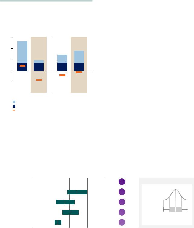
The ten-year outlook for global equities, similar to last year, is centered in the 4.5%–6.5% range based on our Vanguard Capital Markets Model (VCMM) projections.
Expected returns for the U.S. stock market are lower than those for international markets, underscoring the benefits of global equity strategies in this environment.
Equity valuations and Vanguard’s “fair-value” CAPE
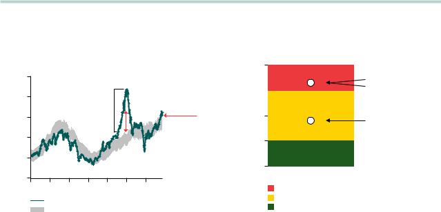
As discussed in a Vanguard Global Macro Matters piece titled As U.S. Stock Prices Rise, the Risk-Return Trade-off Gets Tricky, price/earnings ratios—including Robert Shiller’s cyclically adjusted P/E ratio (CAPE)—are at alarming levels. The current CAPE level corresponds to the 95th percentile of its historical range of values, approaching highs seen during the dot-com era. However, a straight comparison of CAPE (or other valuation multiples) with its historical averages can be misleading, failing to account for today’s low inflation and interest rates.
Because a secular decline in interest rates and inflation depresses the discount rates used in asset-pricing models, investors are willing to pay a higher price for future earnings, thus inflating P/E ratios. Therefore, a high CAPE may not be indicating overvalued stock prices but rather may be an outcome of low inflation and interest rates.
Vanguard’s fair-value CAPE accounts for current interest rates and inflation levels and provides a more useful time-varying benchmark against which the traditional CAPE ratios can be compared, instead of the popular use of historical average benchmarks.
31
vk.com/id446425943
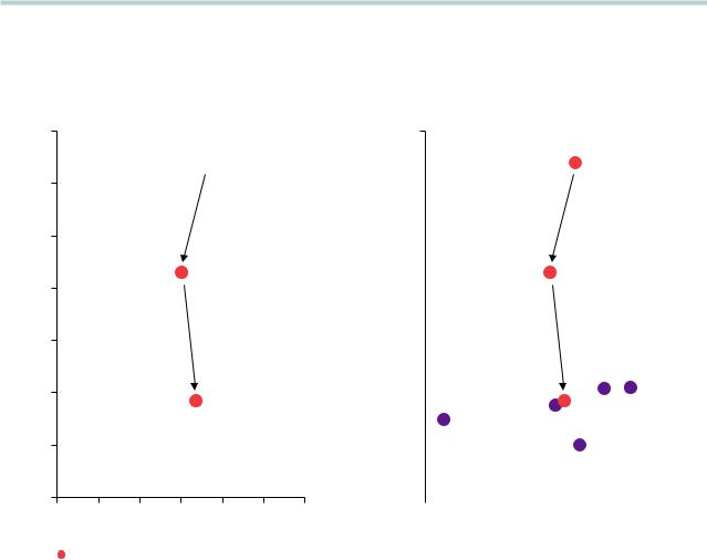
Figure II-1a plots Shiller’s CAPE versus our fair-value model. For instance, in the late 1990s, the difference between the CAPE and our fair-value estimate would have suggested a bubble. Today, although the CAPE is approaching historical highs, it’s not grossly overvalued, as it would be in a bubble, when compared with its fair value.
We have extended this fair-value concept to other regions. As illustrated in Figure II-1b, our equity valuation dashboard indicates that non-U.S. developed markets are fairly valued, even after adjusting valuations for rates and inflation. For emerging markets, it is important to note that their stocks typically trade at lower multiples than those in developed markets because of the higher
FIGURE II-1
Divergence in global equity valuations
a. CAPE for the U.S. S&P 500 Index is approaching overvalued territory
|
|
50 |
|
|
|
|
|
|
Cyclically adjusted |
price/earnings ratio |
40 |
|
|
|
|
|
|
|
|
|
Dot-com |
|
|
|||
30 |
|
|
bubble |
|
|
|||
|
|
|
|
|
|
|||
20 |
|
|
|
|
|
|
||
10 |
|
|
|
|
|
|
||
|
|
|
|
|
|
|
|
|
|
|
0 |
|
|
|
|
|
|
|
|
1950 |
1960 |
1970 |
1980 |
1990 |
2000 |
2010 |
|
|
|
CAPE |
|
|
|
|
|
Fair-value CAPE +/–0.5 standard error
Overvalued, but not
a bubble
Notes: Fair-value CAPE is based on a statistical model that corrects CAPE measures for the level of inflation expectations and for lower interest rates. The statistical model specification is a three-variable vector error correction (VEC), including equity earnings yields, ten-year trailing inflation, and ten-year U.S. Treasury yields estimated over the period January 1940–September 2018.
Source: Vanguard calculations, based on data from Robert Shiller’s website (aida.wss.yale.edu/~shiller/data.htm), the U.S. Bureau of Labor Statistics, and the Federal Reserve Board.
risk and higher earnings yield required by investors. Even after adjusting for higher risk, emerging markets are overvalued.
Global equities and the diversification of domestic risks
As shown in Figure II-2, our expected return outlook for U.S. equities over the next decade is centered
in the 3%–5% range, in stark contrast with the 10.6% annualized return generated over the last 30 years. Although valuation expansion proved to be a tailwind to returns over those 30 years, we expect valuations to contract as interest rates gradually rise over the next decade. The expected equity risk premium (over cash) for the U.S. market appears compressed, primarily because of elevated valuations today.
b. Ex-U.S. developed markets appear to be fairly priced
100
|
|
|
|
Emerging markets |
percentileValuation |
valuefairtorelative |
75 |
|
United States |
|
|
|||
|
|
|
|
50
Ex-U.S. developed markets
25
0
Equity markets
Stretched
Fairly valued
Undervalued
Notes: The U.S. valuation measure is the current CAPE percentile relative to fair-value CAPE for the S&P 500 Index from January 1940–September 2018. The developed markets valuation measure is the weighted average of each region’s (Australia, United Kingdom, Germany, Japan, and Canada) current CAPE percentile relative to its own fair-value CAPE. The fair-value CAPE for the regions is a fivevariable vector error correction (VEC) with equity earnings yield (MSCI index), tenyear trailing inflation, ten-year government bond yield, equity volatility, and bond volatility estimated over the period January 1970 to September 2018. The emerging markets valuation measure is a composite of emerging markets-to-U.S. relative valuations and current U.S. CAPE percentile relative to fair-value CAPE. The relative valuation is the current ratio of emerging markets-to-U.S. price-to-earnings metrics relative to its historical average, using three-year trailing average earnings from January 1990 to September 2018.
Source: Vanguard calculations, based on data from Robert Shiller’s website (aida. wss.yale.edu/~shiller/data.htm), the U.S. Bureau of Labor Statistics, the Federal Reserve Board, and Thomson Reuters Datastream.
32
vk.com/id446425943
FIGURE II-2
The outlook for equity markets is subdued
a. Exposure to non-U.S. equities may be beneficial
U.S. equity |
Global ex-U.S. |
|
equity in U.S. dollars |
|
12% |
return |
8 |
|
|
Annualized |
4 |
0 |
|
|
–4 |
Last |
Next |
Last |
Next |
30 years |
10 years |
30 years |
10 years |
Equity risk premium
Cash return
Valuation expansion/contraction (%)
From a U.S. investor’s perspective, the expected return outlook for non-U.S. equity markets is in the 6%–8% range, modestly higher than that of U.S. equity (Figures II-2a and II-2b). The equity risk premium for
non-U.S. equity markets, however, may be slightly higher going forward, as the valuation contraction may not be as drastic as that experienced over the last three decades.
This result is a function of the currently moderate level of valuations, as well as long-term expectations of the U.S. dollar decline priced in by the markets, especially with respect to other major currencies such as the euro and yen.
Our ten-year outlook for global equity (in USD) is in the 4.5%–6.5% range, as seen in Figure II-2b. Although the case for global diversification is particularly strong now, for the purposes of asset allocation we caution investors against implementing tactical tilts based on just the median expected return—that is, ignoring the entire distribution of asset returns and their correlations.
Notes: Data for the last 30 years are from January 1988–December 2017, in USD. Next-10-year data are based on the median of 10,000 simulations from VCMM
as of September 30, 2018, in USD. Historical returns are computed using indexes defined in “Indexes used in our historical calculations” on page 5. See Appendix for further details on asset classes shown here.
Source: Vanguard calculations, based on data from Dimson-Marsh-Staunton Global Returns Dataset, FactSet, Morningstar Direct, and Thomson Reuters Datastream.
b. Equity market ten-year return outlook: Setting reasonable expectations
|
|
|
|
|
|
|
|
|
|
|
|
|
|
|
|
|
|
|
|
|
|
|
|
|
Median |
|
|
|
|
|
|
|
|
|
|
|
|
|
|
|
|
|
|
|
|
|
|
|
|
|
|
volatility (%) |
|
|
|
|
|
|
|
|
|
|
|
|
|
|
|
|
|
|
|
|
|
|
|
|
|
|
|
|
|
|
|
|
|
|
|
|
|
|
|
|
|
|
|
|
|
|
|
|
|
|
|
|
|||
U.S. REITs |
|
|
|
|
|
|
|
|
|
|
|
|
|
|
|
|
|
|
|
|
|
|
18.4 |
|
||
|
|
|
|
|
|
|
|
|
|
|
|
|
|
|
|
|
|
|
|
|
|
|
|
|||
Global equities ex-U.S. |
|
|
|
|
|
|
|
|
|
|
|
|
|
|
|
|
|
|
|
|
|
18.2 |
|
|||
|
|
|
|
|
|
|
|
|
|
|
|
|
|
|
|
|
|
|
|
|
|
|||||
(unhedged) |
|
|
|
|
|
|
|
|
|
|
|
|
|
|
|
|
|
|
|
|
|
|
||||
|
|
|
|
|
|
|
|
|
|
|
|
|
|
|
|
|
|
|
|
|
|
|
||||
|
|
|
|
|
|
|
|
|
|
|
|
|
|
|
|
|
|
|
|
|
|
|
|
|
|
|
U.S. equities |
|
|
|
|
|
|
|
|
|
|
|
|
|
|
|
|
|
|
|
|
|
|
16.3 |
|
||
|
|
|
|
|
|
|
|
|
|
|
|
|
|
|
|
|
|
|
|
|
|
|
||||
Global equities |
|
|
|
|
|
|
|
|
|
|
|
|
|
|
|
|
|
|
|
|
|
15.8 |
|
|||
|
|
|
|
|
|
|
|
|
|
|
|
|
|
|
|
|
|
|
|
|
|
|||||
|
|
|
|
|
|
|
|
|
|
|
|
|
|
|
|
|
|
|
|
|
|
|||||
In ation |
|
|
|
|
|
|
|
|
|
|
|
|
|
|
|
|
|
|
|
|
|
2.4 |
|
|||
|
|
|
|
|
|
|
|
|
|
|
|
|
|
|
|
|
|
|
|
|
|
|||||
|
|
|
|
|
|
|
|
|
|
|
|
|
|
|
|
|
|
|
|
|
|
|||||
|
|
|
|
|
|
|
|
|
|
|
|
|
|
|
|
|
|
|
|
|
|
|
|
|
|
|
|
|
|
|
|
|
|
|
|
|
|
|
|
|
|
|
|
|
|
|
|
|
|
|
|
|
|
–5 |
0 |
|
|
|
|
5 |
|
10 |
|
|
|
15% |
|
|
|
|||||||||||
|
|
|
|
|
|
|
|
|
|
Ten-year annualized return |
|
|
|
|
|
|||||||||||
Percentile key
|
|
50% |
|
|
Cumulative |
25% |
75% |
||
probability of |
||||
|
|
|
||
lower return 5% |
|
|
95% |
|
Percentiles |
|
|
|
|
5th |
25th |
75th Median |
95th |
|
Notes: Forecast corresponds to distribution of 10,000 VCMM simulations for ten-year annualized nominal returns as of September 30, 2018, in USD, for asset classes shown. Median volatility is the 50th percentile of an asset class’s distribution of annual standardized deviation of returns. See Appendix for further details on asset classes shown here.
Source: Vanguard.
33
vk.com/id446425943
Global fixed income markets: An improved outlook
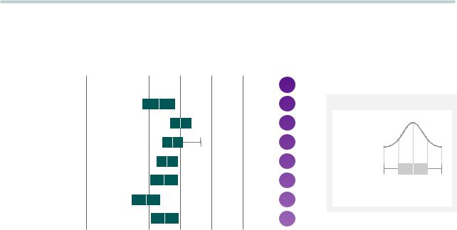
Higher interest rates have improved our outlook for fixed income compared with this time last year. As shown in Figure II-3, it is in the 2.5%–4.5% range for the next decade. Expected returns for the riskier fixed income sub-asset classes appear more differentiated compared with previous years, in part because of
a recent expansion in credit spreads, thereby giving them the cushion to capture the risk premium.
U.S. interest rates: A slightly higher yield curve
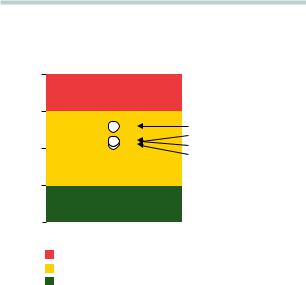
Despite the expected increase in short-term policy rates, the risk of a material rise in long-term interest rates remains modest. As illustrated in Figure II-4,
duration strategies are fairly valued and less risky than investors may believe in a rising rate environment. This is because we expect the short end of the yield curve to rise more than the long end over the next decade, as the long rates are anchored by inflation expectations.
Corporate bonds: Higher risk, higher return
The central tendency for U.S. credit bonds (specifically, the Bloomberg Barclays U.S. Credit Bond Index) is
in the 3.0%–5.0% range, modestly higher than last year because of the rise in the underlying Treasury rates. The central tendency for high-yield corporate bonds (specifically, the Bloomberg Barclays U.S. High Yield Corporate Bond Index) is in the 3.5%–5.5% range, again,
FIGURE II-3
Higher rates have pushed expected fixed income returns higher
|
|
|
|
|
|
|
|
|
|
|
|
|
|
|
|
|
|
|
|
|
|
|
|
|
|
|
|
|
|
|
|
|
|
|
|
|
|
|
|
|
|
|
|
Median |
|
|
|
|
|
|
|
|
|
|
|
|
|
|
|
|
|
|
|
|
|
|
volatility (%) |
|
|
|
|
|
|
|
|
|
|
|
|
|
|
|
|
|
|
|
|
|
|
|
|
U.S. high-yield bonds |
|
|
|
|
|
|
|
|
|
|
|
|
|
|
|
|
|
|
|
10.9 |
|
|
|
|
|
|
|
|
|
|
|
|
|
|
|
|
|
|
|
|
|
|
|||
|
|
|
|
|
|
|
|
|
|
|
|
|
|
|
|
|
|
|
|
|||
|
|
|
|
|
|
|
|
|
|
|
|
|
|
|
|
|
|
|
|
|
|
|
U.S. TIPS |
|
|
|
|
|
|
|
|
|
|
|
|
|
|
|
|
7.7 |
|
||||
|
|
|
|
|
|
|
|
|
|
|
|
|
|
|
|
|
||||||
|
|
|
|
|
|
|
|
|
|
|
|
|
|
|
|
|
||||||
|
|
|
|
|
|
|
|
|
|
|
|
|
|
|
|
|
|
|
|
|
|
|
U.S. credit bonds |
|
|
|
|
|
|
|
|
|
|
|
|
|
|
|
|
|
6.6 |
|
|||
|
|
|
|
|
|
|
|
|
|
|
|
|
|
|
|
|
|
|||||
|
|
|
|
|
|
|
|
|
|
|
|
|
|
|
|
|
|
|||||
|
|
|
|
|
|
|
|
|
|
|
|
|
|
|
|
|
|
|
|
|
|
|
U.S. bonds |
|
|
|
|
|
|
|
|
|
|
|
|
|
|
|
|
5.3 |
|
||||
|
|
|
|
|
|
|
|
|
|
|
|
|
|
|
|
|
||||||
|
|
|
|
|
|
|
|
|
|
|
|
|
|
|
|
|
||||||
U.S. Treasury bonds |
|
|
|
|
|
|
|
|
|
|
|
|
|
|
|
|
|
|
|
|
|
|
|
|
|
|
|
|
|
|
|
|
|
|
|
|
|
|
|
|
|
5.3 |
|
||
|
|
|
|
|
|
|
|
|
|
|
|
|
|
|
|
|
|
|
|
|||
|
|
|
|
|
|
|
|
|
|
|
|
|
|
|
|
|
|
|
|
|||
|
|
|
|
|
|
|
|
|
|
|
|
|
|
|
|
|
|
|
|
|
|
|
Non-U.S. bonds (hedged) |
|
|
|
|
|
|
|
|
|
|
|
|
|
|
|
|
3.7 |
|
||||
|
|
|
|
|
|
|
|
|
|
|
|
|
|
|
|
|
||||||
|
|
|
|
|
|
|
|
|
|
|
|
|
|
|
|
|
||||||
In ation |
|
|
|
|
|
|
|
|
|
|
|
|
|
|
|
|
|
|
|
|
|
|
|
|
|
|
|
|
|
|
|
|
|
|
|
|
|
|
|
|
|
2.4 |
|
||
|
|
|
|
|
|
|
|
|
|
|
|
|
|
|
|
|
|
|
|
|
||
|
|
|
|
|
|
|
|
|
|
|
|
|
|
|
|
|
|
|
|
|
||
|
|
|
|
|
|
|
|
|
|
|
|
|
|
|
|
|
|
|
|
|
|
|
Cash |
|
|
|
|
|
|
|
|
|
|
|
|
|
|
|
|
1.3 |
|
||||
|
|
|
|
|
|
|
|
|
|
|
|
|
|
|
|
|
||||||
|
|
|
|
|
|
|
|
|
|
|
|
|
|
|
|
|
||||||
|
|
|
|
|
|
|
|
|
|
|
|
|
|
|
|
|
|
|
|
|
|
|
|
|
|
|
|
|
|
|
|
|
|
|
|
|
|
|
|
|
|
|
|||
–2 |
0 |
|
2 |
|
|
4 |
|
6 |
8% |
|
|
|
||||||||||
|
|
|
|
|
|
|
|
Ten-year annualized return |
|
|
|
|
|
|||||||||
Percentile key
|
|
50% |
|
|
Cumulative |
25% |
75% |
||
probability of |
||||
|
|
|
||
lower return 5% |
|
|
95% |
|
Percentiles |
|
|
|
|
5th |
25th |
75th Median |
95th |
|
Notes: Forecast corresponds to distribution of 10,000 VCMM simulations for ten-year annualized nominal returns as of September 30, 2018, in USD for asset classes shown. Median volatility is the 50th percentile of an asset class’s distribution of annual standardized deviation of returns. See Appendix for further details on asset classes shown here.
Source: Vanguard.
34
vk.com/id446425943
FIGURE II-4
Fixed income appears to be fairly valued
percentile |
100 |
|
75 |
U.S. aggregate bonds |
|
|
|
|
|
|
Intermediate credit |
|
|
Duration strategy |
Valuation |
50 |
TIPS |
|
||
25 |
|
|
|
|
0
Bond markets
Stretched
Fairly valued
Undervalued
Notes: Valuation percentiles are relative to Year 30 projections from VCMM. Intermediate credit and U.S. aggregate bond valuations are current spreads relative to Year 30 from VCMM. Duration valuation is the expected return differential over the next decade between the long-term Treasury index and the short-term Treasury index relative to Years 21–30. The TIPS valuation is the ten-year-ahead annualized inflation expectation relative to Years 21–30.
Source: Vanguard.
higher because of higher underlying Treasury rates. We urge investors to be cautious in reaching for yield in segments such as high-yield corporates, not only because of the higher expected volatility that accompanies the higher yield but also because of the segment’s correlation to the equity markets.
As shown in Figure II-5 (on page 37), a 20% overweight or tilt to high-yield corporates increases a portfolio’s volatility excessively relative to a marginal increase in return. The sensitivity of spreads to the economic
environment is much larger for high-yield corporate bonds than for other higher-quality segments of the U.S. fixed income market, which also contributes to an increased investment risk.
Treasury Inflation-Protected Securities (TIPS): Markets don’t see inflation coming
Break-even inflation expectations inferred from the U.S. TIPS market remain close to the Fed’s 2% inflation target and the VCMM long-term median levels. Markets are placing low odds for higher inflation outcomes. Although not attractive from
a return perspective, TIPS could be a valuable inflation hedge for some institutions and investors sensitive to inflation risk.
Domestic versus international: Benefits of diversification remain
Although the central tendency of expected return
for non-U.S. aggregate bonds appears to be marginally lower than that of U.S. aggregate bonds (see Figure II-3 on page 34), we expect the diversification benefits
of global fixed income in a balanced portfolio to persist under most scenarios.
Yields in most developed markets are historically low, particularly in Europe and Japan, yet diversification through exposure to hedged non-U.S. bonds should help offset some risk specific to the U.S. fixed income market (Phillips et al., 2014).
Less-than-perfect correlation between two of the main drivers of bond returns—interest rates and inflation—is expected as global central bank policies are likely to diverge in the near term. Diversification with non-U.S. bonds also helps diversify the risk
of policy mistakes by central banks.
35
vk.com/id446425943
Portfolio implications: A low return orbit
Investors have experienced spectacular returns over the last few decades because of two of the strongest equity bull markets in U.S. history, in addition to a secular decline in interest rates from 1980s highs. Figure II-5a contrasts our 4%–6% outlook for a global 60% equity/40% bond portfolio for the next decade against the extraordinary 9.4% return since 1970 and the 7.3% return since 1990. As highlighted in previous sections, elevated equity valuations and low rates have pulled the market’s efficient frontier of expected returns into a lower orbit. The efficient frontier is also flatter (that is, with less return per unit of risk), as seen from the return and volatility expectations of balanced portfolios, as shown in Figure II-5c.
To try to increase portfolio returns, a popular strategy
is to overweight higher-expected-return assets or higheryield assets. A common “reach for yield” strategy is to overweight high-yield corporates. Similarly, “reach for return” strategies involve tilting the portfolio toward emerging-market equities to take advantage of higher growth prospects. Home bias causes some to shy away from non-U.S. equities.
Figure II-5b illustrates that these common return-centric strategies are unlikely, by themselves, to restore portfolios to the higher orbit of historical returns.
36
vk.com/id446425943
FIGURE II-5
Asset allocation for a challenging decade
a. A lower return orbit …
10%
 Since 1970
9
8
Since 1990
7
Return
6
5
Next decade
4
3
6 |
7 |
8 |
9 |
10 |
11 |
12% |
|
|
|
Volatility |
|
|
|
b.… that popular “active tilts” will likely fail to escape
10%
9 |
|
|
|
|
|
|
|
|
|
|
|
|
|
|
|
|
|
|
|
|
|
|
|
|
|
|
|
8 |
|
|
|
|
|
|
|
|
|
|
|
|
|
|
|
|
|
|
|
|
|
|
|
|
|
|
|
7 |
|
|
|
|
|
|
|
|
|
|
|
|
|
|
|
|
|
|
|
|
|
|
|
|
|
|
|
Return |
|
|
|
|
|
|
|
|
|
|
|
||
6 |
|
|
|
|
|
|
|
|
|
High- |
|
|
|
|
|
|
|
|
|
|
|
|
|
|
|||
|
|
|
|
|
|
|
|
|
|
|
|
||
|
|
|
|
|
|
|
|
|
|
yield |
|
|
|
|
|
|
|
|
|
|
|
|
|
tilt |
|
|
|
5 |
|
|
U.S. |
|
|
|
|
|
|
|
|
|
|
|
|
cash |
|
|
|
|
|
|
Emerging |
||||
|
|
|
|
|
|
|
|
|
|||||
|
|
|
tilt |
|
TIPS |
|
|
|
markets |
||||
|
|
|
|
|
|
|
|
|
equity tilt |
||||
|
|
|
|
|
|
tilt |
|
|
|
|
|
|
|
4 |
|
|
|
|
|
|
|
60/40 without |
|
|
|||
|
|
|
|
|
|
|
|
|
|||||
|
|
|
|
|
|
|
|
|
|
||||
|
|
|
|
|
|
|
|
ex-U.S. equity |
|
|
|||
3 |
|
|
|
|
|
|
|
|
|
|
|
|
|
|
|
|
|
|
|
|
|
|
|
|
|
|
|
6 |
7 |
8 |
9 |
10 |
11 |
12% |
|||||||
Volatility
Global 60% equity/40% bond portfolio
c. Projected ten-year annualized nominal returns as of September 2018
|
|
|
25th |
|
75th |
95th |
Median |
|
|
Portfolios 5th percentile |
percentile |
Median |
percentile |
percentile |
volatility |
||
|
|
|
|
|
|
|
|
|
|
100% bonds |
1.8% |
2.7% |
3.4% |
4.1% |
5.1% |
4.5% |
|
Global |
20/80 stock/bond |
2.3% |
3.3% |
4.0% |
4.7% |
5.9% |
4.5% |
|
balanced |
60/40 stock/bond |
1.5% |
3.5% |
4.9% |
6.3% |
8.4% |
9.4% |
|
portfolios |
80/20 stock/bond |
0.8% |
3.4% |
5.2% |
7.0% |
9.7% |
12.5% |
|
|
|
|
|
|
|
|
|
|
|
100% equity |
–0.1% |
3.1% |
5.3% |
7.6% |
11.0% |
15.8% |
|
|
60/40 stock/bond |
1.5% |
3.5% |
4.9% |
6.3% |
8.4% |
9.4% |
|
|
|
|
|
|
|
|
|
|
Portfolios |
High-yield tilt |
1.8% |
3.7% |
5.1% |
6.5% |
8.7% |
10.4% |
|
|
|
|
|
|
|
|
||
Inflation protection tilt |
1.4% |
3.4% |
4.8% |
6.2% |
8.4% |
9.2% |
||
with common |
||||||||
20% tilts |
Emerging markets equity tilt |
1.4% |
3.6% |
5.1% |
6.6% |
8.8% |
11.0% |
|
relative to 60/40 |
U.S. cash tilt |
1.9% |
3.4% |
4.4% |
5.5% |
7.1% |
6.4% |
|
stock/bond |
|
|
|
|
|
|
|
|
60/40 without ex-U.S. equity |
0.1% |
2.5% |
4.0% |
5.6% |
8.1% |
9.8% |
||
|
||||||||
Notes: The figure shows summary statistics of 10,000 VCMM simulations for projected ten-year annualized nominal returns as of September 2018 in USD before costs. Historical returns are computed using indexes defined in “Indexes used in our historical calculations” on page 5. The global equity portfolio is 60% U.S. equity and 40% global ex-U.S. equity. The global bond portfolio is 70% U.S. bonds and 30% global ex-U.S. bonds. Portfolios with tilts include a 20% tilt to the asset specified funded from the fixed income allocation for the fixed income tilts and the equity allocation for the equity tilts.
Source: Vanguard.
37

vk.com/id446425943
Portfolio construction strategies
for three potential economic scenarios
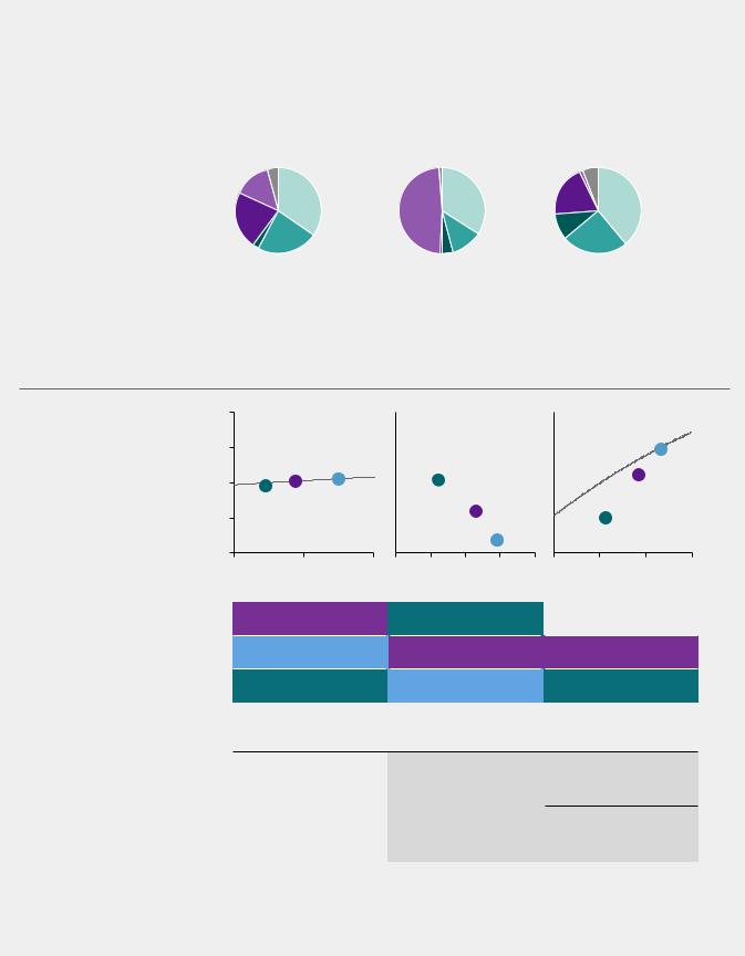
Based on our global economic perspective, we examine in Figure II-6 three possible economic scenarios occurring over the next three years. The high-growth scenario illustrates an upside risk scenario of sustained economic growth with tighter labor markets and a moderate pickup in wages and inflation. The two others are a status quo scenario driven by continued low volatility with positive financial conditions and a recessionary scenario caused by a turn in the business cycle and a correction in the equity markets.
Figure II-6 shows optimal portfolios for each scenario that vary their exposures to the following four factors, or risk premiums: equity risk premium, term premium, credit premium, and inflation-risk premium. In a highgrowth scenario, expected global equity returns would be high, causing the efficient frontier to be steep. Long and short rates would also rise faster than expected, resulting in an optimal portfolio loading on equity and short duration.
A recessionary-scenario portfolio would underweight equity and overweight long duration. Surprisingly, the allocation to U.S. equity remains rather large, as the portfolio that is also heavy on long-term Treasuries derives a larger diversification benefit from lower-returning U.S. equity (especially in a recession) than from including higher-returning non-U.S. equity assets. The portfolio strategy in a status quo scenario is well-diversified.
Using our VCMM simulations, we are able not only to illustrate the effectiveness of various portfolio strategies designed for each scenario but also to show the risks of such strategies. The following conclusions can be drawn from our analysis:
1.Portfolios designed for specific macroeconomic scenarios entail important trade-offs: If the scenario for which the portfolio was designed does not take place, then the portfolio performance is the worst of all the options.
2.A balanced portfolio works well for investors who are agnostic about the future state of the economy: The 60/40 balanced portfolio
is an “all-weather” strategy, with either top or middle-of-the-road performance in each scenario.
3.Portfolio tilts should be done within an optimization framework: Ad hoc tilts ignore correlations among assets and lead to inefficient portfolios. For instance, in a recession-scenario strategy, U.S. equities
can be relatively overweighted (as opposed to underweighted) because of the added diversification benefits of long-term bonds.
38
vk.com/id446425943
FIGURE II-6
Cyclical surprises and asset allocation trade-offs
a. Optimal portfolios |
Scenario 1 |
Scenario 2 |
Scenario 3 |
vary for different |
Status quo/baseline |
Recession |
High growth |
economic |
Diversi ed |
Overweight long duration |
Overweight equity |
environments |
|||
|
portfolio |
and underweight equity |
and short duration |
|
35% |
U.S. equity |
|
34% |
U.S. equity |
|
39% |
U.S. equity |
|
|
|
||||||
|
23% |
Global ex-U.S. equity |
|
12% Global ex-U.S. equity |
|
25% |
Global ex-U.S. equity |
|
|
|
|
||||||
|
2% |
Global ex-U.S. bonds |
|
4% |
Global ex-U.S. bonds |
|
10% |
Global ex-U.S. bonds |
|
|
|
||||||
|
0% |
Short-term credit |
|
0% |
Short-term credit |
|
0% |
Short-term credit |
|
|
|
||||||
|
22% |
Short-term Treasury |
|
1% |
Short-term Treasury |
|
19% |
Short-term Treasury |
|
|
|
||||||
|
14% |
Long-term Treasury |
|
48% |
Long-term Treasury |
|
1% |
Long-term Treasury |
|
|
|
||||||
|
4% |
Short-term TIPS |
|
1% |
Short-term TIPS |
|
6% |
Short-term TIPS |
|
|
|
||||||
b. A diversified |
|
8% |
|
|
|
|
|
|
|
|
|
|
return |
6 |
|
|
|
|
|
|
|
|
|
|
|
portfolio is not |
|
|
|
|
|
|
|
|
|
|
||
|
|
|
|
|
|
|
|
|
|
|
|
|
always the best, but |
annualized |
|
|
|
|
|
|
|
|
|
|
|
it’s never the worst |
4 |
|
|
|
|
|
|
|
|
|
|
|
|
|
|
|
|
|
|
|
|
|
|
||
|
|
|
|
|
|
|
|
|
|
|
|
|
|
Median |
2 |
|
|
|
|
|
|
|
|
|
|
|
0 |
|
|
|
|
|
|
|
|
|
|
|
|
|
|
|
|
|
|
|
|
|
|
|
|
|
|
6 |
7 |
8% |
6 |
8 |
10 |
12 |
14% 4 |
6 |
8 |
10% |
|
|
|
|
|
|
Median volatility |
|
|
|
|
||
Best |
Diversified |
Overweight long duration |
Overweight equity |
|
portfolio |
and underweight equity |
and short duration |
|
|
|
|
|||
|
|
|
|
|
Second-best |
Overweight equity |
Diversified |
Diversified |
|
and short duration |
portfolio |
portfolio |
|
|
|
|
|||
Worst |
Overweight long duration |
Overweight equity |
Overweight long duration |
|
and underweight equity |
and short duration |
and underweight equity |
|
|
|
|
|||
|
|
|
|
|
c.Portfolios designed for a single scenario are tempting but can be risky
Strategy upside relative |
1.4% higher annualized |
to balanced portfolio |
return with 2.1% lower |
|
volatility in a recessionary |
|
scenario |
|
|
Strategy downside relative |
1.8% lower annualized |
to balanced portfolio |
return with 1.4% lower |
|
volatility in a high-growth |
|
scenario |
|
|
1.1% higher annualized return with 1.1% higher volatility in a high-growth scenario
1.2% lower annualized return with 1.2% lower volatility in a a recessionary scenario
Notes: Performance is relative to the efficient frontier. Portfolios are selected from the frontier based on a fixed risk-aversion level using a utility function-based optimization model. The forecast displays a simulation of three-year annualized returns of asset classes shown as of September 2018. Scenarios are derived from sorting the VCMM simulations based on rates, growth, volatility, and equity return. The three scenarios are a subset of the 10,000 VCMM simulations. See Appendix for further details on asset classes shown here.
Source: Vanguard.
39
vk.com/id446425943
Portfolio construction strategies: Time-tested principles apply
Contrary to suggestions that an environment of low rates and compressed equity risk premiums warrants some radically new investment strategy, Figure II-5 (on page 37) reveals that the diversification benefits of global fixed income and global equity are particularly compelling, given the simulated ranges of portfolio returns and volatility.
The market’s efficient frontier of expected returns for a unit of portfolio risk is in a lower orbit. More important, common asset-return-centric portfolio tilts,
seeking higher return or yield, are unlikely to escape the strong gravity of low-return forces in play, as they ignore the benefits of diversification. Modestly outperforming asset-return-centric tilts requires a portfolio-centric approach that leverages the benefits of diversification by weighing risk, return, and correlation simultaneously.
Our prior research shows that investment success is within the control of long-term investors (Aliaga-Díaz, et al., 2016). Factors within a long-term investor’s
control—such as saving more, working longer, spending less, and controlling investment costs—far outweigh the less reliable benefits of ad hoc asset-return-seeking tilts. Thus, decisions around saving more, spending less, and controlling costs will be much more important than portfolio tilts.
Investment objectives based either on fixed spending requirements or on fixed portfolio return targets may require investors to consciously weigh their options in conjunction with their risk-tolerance levels. Ultimately, our global market outlook suggests a somewhat more challenging environment ahead, yet one in which investors with an appropriate level of discipline, diversification, and patience are likely to be rewarded over the long term. Adhering to investment principles such as long-term focus, disciplined asset allocation, and periodic portfolio rebalancing will be more crucial than ever before.
40