

Учебники / Hair Cell Regeneration, Repair, and Protection Salvi 2008
.pdf82 J.C. Saunders and R.J. Salvi
LOW FREQUENCY
apex
neural |
abneural |
Most Neural |
Neural |
base |
Medial |
Abneural |
HC |
HC |
|
HC |
HC |
HIGH FREQUENCY
Figure 3.2. This cartoon depicts the innervation and organization of chick neural (left side) and abneural (right side) hair cells. The afferent fibers are colored black while efferent fibers are indicated by the speckles. (Modified from Fisher 1994, with permission.)
Changes occur in hair cell innervation from the abneural to neural edges of the papilla. The abneural hair cells have large efferent endings and minimal size afferent endings. Neural hair cells exhibit large afferent endings with small efferent terminals (Fig. 3.2). Depending on location, the number of afferent fibers that innervate each neural hair cell is between 1.4 and 2.4 (Fig. 3.2).
Ototrauma from loud sound or ototoxic drugs results in hair cell loss, which inevitably means that the neural connections with the hair cell are broken. These connections must repair themselves if auditory function is to return to normal (Ryals and Dooling 1996). Issues such as the postexposure fate of synaptic boutons, the degree of axonal degeneration and recovery, the mechanisms that guide neurons back to their correct tonotopic location, the time course of neural recovery, and the importance of innervation in inducing hair cell regeneration are far from well understood. Indeed, it has been a vexing question to clearly trace the degeneration and/or recovery of afferent and efferent neurons after ototrauma.
3. Recovery of Function |
83 |
Transmission electron microscopy of serial sections, antibody labeling of neurofilament proteins in axons, and the application of synapsin or syntaxinspecific immunohistochemistry, have been used to gain some idea of the loss and recovery of afferent and efferent elements in the cochlear nerve. Four scenarios for the fate of cochlear neurons have been proposed (Cotanche et al. 1994):
(1) The axons remain connected to the synaptic bouton, and the bouton itself separates from the dying hair cell. In this situation the neural elements remain in place, and simply await the reemergence of new hair cells with which to make contact. (2) The afferent and efferent terminals remain attached to the hair cell with the more central axon projection breaking off. Despite the loss of the synaptic terminal, as the hair cell degenerates, the nerve fibers remain intact, healthy, and in position. In this case the sprouting of new terminals would be required for reinnervation with new hair cells. (3) The synaptic endings of the neurons are lost, which leads to degeneration of afferent and efferent fibers. As these fibers degenerate they retract toward the cochlear ganglion cell body. Repair, in this situation, would require axonal regrowth, and the formation of a new synaptic bouton before reinnervation could occur. (4) Axonal degeneration might be so severe that it leads to the loss of ganglion cell bodies, and in this scenerio repair might be impossible.
Synapses have been observed on newly regenerated hair cells 3–4 days after acoustic trauma, indicating that reinnervation does indeed take place (Ryals and Dooling 1996). Moreover, neurofilament labeling of the cochlear nerve, in moderately damaged ears, revealed that the synaptic endings, while separated from the axon, appeared to remain attached to dying hair cells. The axons, even though separated from the bouton, remain in the immediate vicinity of the hair cells to which they were originally connected (Ofsie and Cotanche 1996; Ofsie et al. 1997). In addition, there was no apparent loss in the number of fibers or their pattern of distribution on the papilla. The tonotopic specificity of the papilla remained intact, and this was supported by fiber tracing, which revealed the papilla frequency map unchanged after hair cell regeneration (Chen et al. 1996). It has also been reported that efferent fibers remained in contact with surviving hair cells in the lesion, implying that the afferent connections on these cells were also intact.
Immunolabeling of the papilla with synapsin, a marker for small synaptic vesicles in neurons, indicated that new hair cells were not initially associated with the presence of efferent fiber terminals after acoustic overstimulation (Ofsie et al. 1997). However, within 7 days of the emergence of new hair cells the first efferent terminals were identified, thus providing additional evidence that the presence of nerve endings was not a requisite for the emergence of new hair cells. With severe acoustic damage to the papilla (e.g., damage in which both hair cells and supporting cells are destroyed), there appeared to be a loss of both the synaptic ending and the nerve fiber (Cotanche 1999). The recovery of the cochlear nerve in this situation has yet to be described, but may well take longer and be less effective.
84 J.C. Saunders and R.J. Salvi
The restoration of efferent nerve terminals after gentamicin destruction of hair cells has also been traced (Hennig and Cotanche 1998). The ototoxic recovery of neural connections occurred in several stages and takes longer than after acoustic trauma, which may account for the extended functional recovery reported in these ears (see Section 2.4). There also appeared to be differences in the regeneration of efferent terminals after ototoxic injuries to the papilla, again reflecting the more extensive damage to the sensory surface after aminoglycoside trauma.
2.3 Cochlear Nerve Coding of the Acoustic Stimulus
Access to the cochlear nerve may be achieved via an opening in the bony skull overlying the recussus scala tympani, which reveals the cochlear nerve lying beneath the distal wall of this chamber. Passing a microelectrode through the perilymph and penetrating the wall gains access to cochlear ganglion cells and nerve fibers. Remarkably, opening the scala tympani does not alter cochlear mechanics.
Parameters of the cochlear nerve response can assess various functions of the peripheral ear. These can be organized into categories that include spontaneous activity, threshold sensitivity, frequency selectivity, intensity coding, synchronization or phase locking, transient detection and adaptation, and neuronal suppression. The findings below are largely from the young chick, but they are nearly identical to those reported in the adult animal.
2.3.1 Tuning Curves
Frequency selectivity is most commonly determined through the threshold tuning curve or the response area curve. These curves describe either iso-response or iso-stimulus contours of unit activity at many frequencies. Threshold tuning curves use an algorithm that determines the sound pressure level (SPL) needed to achieve a sound-driven criterion response level of, for example, 2 spikes/s (S/s) above the level of spontaneous activity. When measured at many frequencies, it forms an iso-response contour. The response area curve is an iso-stimulus plot describing discharge activity to a constant intensity tonal stimulus of varying frequency. When the discharge activity produced by a random matrix of tone bursts at different frequency and intensity combinations is reconstructed into a tuning curve, it is referred to as a spectral response plot. Tuning curves reflect not only the frequency selective properties of the inner ear but also the tonotopic distribution of frequency along the sensory epithelium. Auditory nerve fibers have been mapped to their hair cell of origin in the chick and pigeon (Chen et al. 1994; Smolders et al. 1995).
Examples of spectral response plot tuning curves in the chick are seen in Figure 3.3. Tuning curves arise from frequency selective mechanisms acting on or within hair cells. One of these is a traveling wave on the basilar membrane. In birds, the locations of the maximum membrane deflection change with frequency, exhibit tonotopic organization along the length of the membrane, and exhibit
3. Recovery of Function |
85 |
DECIBELS SPL
|
CONTROL |
|
0 - DAY |
|
|
12 - Day |
|||
A |
|
|
B |
|
|
C |
|
|
|
|
|
|
100 |
|
|
|
|
|
|
|
|
|
80 |
|
|
|
|
|
|
|
|
|
60 |
|
|
|
|
|
|
|
|
|
40 |
|
|
|
|
|
|
|
|
|
20 |
|
|
|
|
|
|
0.1 |
0.3 0.6 1.0 |
3.0 |
0.1 |
0.3 0.6 1.0 |
3.0 |
0.1 |
0.3 |
0.61.0 |
3.0 |
FREQUENCY IN KHZ
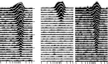
Figure 3.3. (A–C) Three spectral response tuning curves are seen for each of three units with a similar CF. The tuning curves from exposed chicks were obtained at 0 days of recovery (B) or after 12 days of postexposure recovery (C), and should be compared against the age-matched control tuning curve at the equivalent of 0 days of recovery (A). Immediately after removal from the exposure, the CF threshold is elevated and the tuing curve is less frequency selective. The unit recorded after 12 days of recovery is identical to the control unit indicating complete recovery. (Data from Saunders et al. 1996a, with permission.)
relatively poor fequency selectivity (von Békésy et al. 1960; Gummer et al. 1987). If the level of frequency selectivity seen in the basilar membrane response were communicated to the hair cell stereocilia, with no other tuning influence, then the resulting neural tuning curve seen in Figure 3.3A would be much wider. The fact that the cochlear nerve tuning curves are sharper than what would be predicted by the mechanical response of the basilar membrane indicates additional sources of tuning.
A second frequency selective mechanism is found within the hair cell itself, and is associated with electrical tuning of the membrane (Fuchs et al. 1988). Electrical tuning arises from the interaction between voltage-gated Ca2+ and calcium-gated K+ channels and their splice variants. When the movements of the sensory hairs are at the same frequency as the resonance of the hair cell membrane, the magnitude of membrane depolarization is greatest. As a consequence, activity in the cochlear nerves attached to the hair cell is greatest relative to the activity generated by any other frequency at the same level.
Third, a compressive nonlinearity may be due to motor activity that changes the mechanical properties of the sensory hair bundles of the hair cell. This activity might alter the stiffness of the bundle and thus influence hair cell frequency selectivity. Such mechanisms have been identified in anuran ears, but are less
86 J.C. Saunders and R.J. Salvi
well understood in the avian ear (Manley 2000, 2001). The interaction of these three tuning processes, and their precise contributions to frequency selectivity, as measured in cochlear nerve tuning curves, remain to be elucidated.
Three spectral response plots from cochlear nerve units are shown in Figure 3.3: one from a normal control (Fig. 3.3A), another from a noise-exposed chick immediately after acoustic overstimulation (Fig. 3.3B), and a third from a chick 12 days postexposure (Fig. 3.3C). All have a common characteristic frequency (CF), which is the lowest point on the tuning curve where sounddriven activity can be identified (about 1.15 kHz). The example in Figure 3.3B shows the typical loss of CF threshold and the deterioration of frequency selectivity seen shortly after removal from the exposure. The recovery of tuning is apparent in Figure 3.3C.
2.3.2 Threshold Sensitivity, Sharpness of Tuning, and Spontaneous Activity
Additional phenomena can be synthesized from unit tuning curves obtained over a range of CFs. In normal ears, CF thresholds at any given frequency exhibit a range of 30–40 dB from the best to poorest threshold levels. In addition, the sensitivity of the lowest threshold at CFs, across frequency approximate the behavioral threshold curve of the chicken (Gray and Rubel 1985). In young and adult chickens, the absolute threshold of hearing is U shaped with thresholds of approximately 0.1–0.2 kHz and 2.8–4.0 kHz showing the poorest, and those between 0.9 and 1.3 kHz, the best sensitivity. Figure 3.4A shows the CF thresholds in a large sample of units recorded from a group of 3-day-old nonexposed control chicks. Figure 3.4B shows CF thresholds in age-matched units recorded shortly after removal from an intense pure-tone exposure. A comparison of Figures 3.4A and B reveals that units with CFs above 0.4 kHz show threshold shifts corresponding to frequencies near and above the 120 dB SPL exposure tone of 0.9 kHz. The CF thresholds in Figure 3.4B are from units in exposed animals allowed 12 days to recover, and demonstrate completely recovery. The rate of threshold recovery over time is too difficult to trace with single-unit studies, but has been effectively followed using evoked responses directly recorded from the chick brainstem (McFadden and Saunders 1989).
Frequency selectivity is quantified by measuring the Q of the tuning curve. This is an index of filter sharpness defined by the ratio of the characteristic frequency (CF in Hz), divided by the bandwidth of the tuning curve in Hz at a criterion level above the CF (typically 10 dB). Since Q is a ratio, the sharpness of tuning can be directly compared across units with different CFs. The larger the Q value is, the sharper the filter. Figure 3.4D shows Q10dB ratios in cochlear nerve units recorded from 3-day-old control chicks. The value of Q10dB increases (as does the variability) with increasing CF, meaning that frequency selectivity becomes sharper in units originating from higher (more basal) frequency regions of the basilar papilla. Interestingly, the most selective units in birds exhibit sharper tuning than seen at equivalent frequencies in mammals (Manley 2001). Figures 3.4E and F show what happens to frequency selectivity just after removal from an intense sound exposure, and after 12 days of recovery. Tuning curves
|
|
3. Recovery of Function |
87 |
CONTROL |
0 - Day |
12 - Day |
|
DB SPL
Q10 dB
SA IN S/S
100
80 |
|
|
|
|
A |
|
|
|
|
B |
|
|
|
|
C |
|
|
|
|
|
|
|
|
|
|
|
|
|
|
|
|
60 |
|
|
|
|
|
|
|
|
|
|
|
|
|
|
|
40 |
|
|
|
|
|
|
|
|
|
|
|
|
|
|
|
20 |
|
|
|
|
|
|
|
|
|
|
|
|
|
|
|
16 |
|
|
|
|
|
|
|
|
|
|
|
|
|
|
|
14 |
n = 491 |
|
|
D |
n = 336 |
|
|
E |
n = 449 |
|
|
F |
|||
12 |
|
|
|
|
|
|
|
|
|
|
|
|
|
|
|
10 |
|
|
|
|
|
|
|
|
|
|
|
|
|
|
|
8 |
|
|
|
|
|
|
|
|
|
|
|
|
|
|
|
6 |
|
|
|
|
|
|
|
|
|
|
|
|
|
|
|
4 |
|
|
|
|
|
|
|
|
|
|
|
|
|
|
|
2 |
|
|
|
|
|
|
|
|
|
|
|
|
|
|
|
0 |
|
|
|
|
|
|
|
|
|
|
|
|
|
|
|
120 |
|
|
|
|
|
|
|
|
|
|
|
|
|
|
|
100 |
|
|
|
|
G |
|
|
|
|
H |
|
|
|
|
I |
80 |
|
|
|
|
|
|
|
|
|
|
|
|
|
|
|
60 |
|
|
|
|
|
|
|
|
|
|
|
|
|
|
|
40 |
|
|
|
|
|
|
|
|
|
|
|
|
|
|
|
20 |
|
|
|
|
|
|
|
|
|
|
|
|
|
|
|
0 |
|
|
|
|
|
|
|
|
|
|
|
|
|
|
|
-20 |
0.1 |
0.3 |
0.6 |
1.0 |
3.0 |
0.1 |
0.3 |
0.6 |
1.0 |
3.0 |
0.1 |
0.3 |
0.6 |
1.0 |
3.0 |
|
|||||||||||||||
CHARACTERISTIC FREQUENCY IN kHz
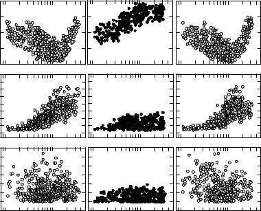
Figure 3.4. (A) Open circles show CF threshold from 491 units in control chicks. (B) The closed circles reveal the same thresholds in 336 units in exposed but 0-day recovered chicks. The threshold shift of units in the 0-day recovery group with CFs between 0.5 and 3.0 kHz is apparent. (C) CF thresholds are plotted for exposed chicks allowed 12 days of postexposure recovery. (D–F) Similarly organized data for frequency selectivity, as measured by the Q10dB metric. (G–I) Data organized for spontaneous activity (SA). A comparison between the control data (A, D, G) with results in exposed units after 12 days of recovery reveals a complete return to normal. (Data from Saunders et al. 1996a, with permission.)
become much broader (have a lower Q) after the exposure, but within 12 days return to normal.
Threshold and tuning were also measured in adult chickens after exposures (48 h, 0.53 kHz, 120 dB SPL) that destroyed hair cells and the tectorial membrane. The CF thresholds were similarly elevated, and iso-response tuning curves were more broadly tuned immediately after the exposure. Threshold and tuning were partially recovered by 5 days postexposure; however, peculiar W-shaped tuning curves with multiple tips and hypersensitive tails, similar to those seen in the developing ear, were also reported (Chen et al. 1996). Single-fiber labeling showed a normal cochlear frequency-place map despite the elevated CF thresholds and broad tuning. After 28 days of recovery, tuning and thresholds were almost normal. Nevertheless, the CF thresholds of the most sensitive
88 J.C. Saunders and R.J. Salvi
neurons were still slightly elevated, tuning curve slopes below CF were shallower than normal, and thresholds in the low-frequency tail of the tuning curves were often hypersensitive. These functional deficits were associated with residual structural damage to the upper fibrous layer of the tectorial membrane over the patch lesion.
Spontaneous activity (SA) represents neuron discharges in the absence of any planned sound stimulation of the ear. This activity arises from the release of neurotransmitter by the hair cell due to Brownian movements of the sensory hair bundles, ambient noise stimulation, and/or spontaneous exocytosis of neurotransmitter vesicles. Spontaneous activity in birds tends to be higher than in mammals, and in some units may be well over 110 S/s. Figure 3.4G shows spontaneous activity in young chicks plotted against CF in control units, and while the SA from unit to unit is quite variable, there is little systematic change across frequency. The consequence of intense sound, just after removal from the exposure, greatly suppresses spontaneous activity (Fig. 3.4H), while Figure 3.4I shows the return of spontaneous activity after 12 days of recovery. Suppression and recovery of spontaneous activity after sound damage has also been observed in adult birds (Chen et al. 1996).
2.3.3 Intensity Coding
Changes in discharge activity with increasing sound intensity describe the rateintensity function. These functions have been reported for the pigeon, owl, emu, starling, and chick. In the chicken, four types of functions have been identified: saturating, sloping upward, straight, and sloping downward (Saunders et al. 2002). Rate-level functions arise from several processes. Changes in stimulus intensity result in different levels of basilar membrane displacement and hence hair bundle displacements. This in turn varies the level of hair cell membrane depolarization, neurotransmitter release, and neuron excitation. While basilar membrane movements with changes in intensity have been described as linear in the pigeon (Gummer et al. 1987), the rate-intensity function shows a compressive nonlinearity at higher stimulus levels. In mammals, OHC contractility is thought to be the principal mechanism of cochlear nonlinearity. There is no evidence of somatic motility in the avian hair cells (He et al. 2003; Köppl et al. 2004). However, this compression may arise from a nonlinearity thought to be associated with the response properties of individual hair cells.
Figures 3.5A–C show rate-level functions for low-, mid-, or high-frequency units (each curve is the average of a number of sloping-up units with a common CF) from control (open circles) and exposed (closed circles) ears shortly after removal from the exposure. At the lowest intensities, only spontaneous activity is seen. Sound-driven responses emerge after a threshold stimulus level is achieved, and discharge activity then increases with sound level (over an approximate 30–40 dB range in control units). Above that range, the slope of the growth
3. Recovery of Function |
89 |
SPIKES PER SECOND
350 |
|
|
|
0.24 kHz |
0.85 kHz |
300 |
0.28 kHz |
0.88 kHz |
250 |
|
|
200 |
|
|
150 |
|
|
100 |
|
|
50 |
|
|
|
A |
B |
0 |
|
|
350 |
|
|
|
0.29 kHz |
0.92 kHz |
300 |
0.32 kHz |
0.89 kHz |
250
200
150
100
50
|
|
|
|
D |
|
|
|
|
E |
0 |
20 |
40 |
60 |
80 100 0 |
20 |
40 |
60 |
80 |
100 |
0 |
DECIBELS SPL
2.39 kHz |
2.53 kHz |
C |
|
2.51 kHz |
|
||
|
2.55 kHz |
|
||
|
|
|
|
F |
0 |
20 |
40 |
60 |
80 100 |
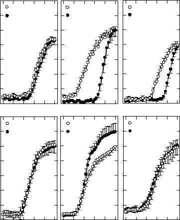
Figure 3.5. (A–C) Rate-level functions for units with the indicated CFs are shown from exposed chicks at 0 days of recovery (black circles) and age-matched nonexposed controls (white circles). The most severe change in the exposed functions occurs near the 0.9-kHz exposure frequency (B) with a pronounced threshold shift and steeper growth of activity. (D–F) Similar data in exposed units 12 days postexposure (black circles) and age-matched control units (white circles) appear. The functions in D and F show complete recovery. Exposed units with CFs near the exposure frequency (E) show a steeper growth segment and a larger discharge rate at the higher intensities. These plots represent the average of 6–9 units, each with the same approximate CF. (Data from Saunders et al., 1996a and Plontke et al. 1999, with permission.)
function becomes shallower. The threshold shift for exposed functions with CFs near the exposure frequency (Fig. 3.5B) is obvious, and the initial growth segment is steeper than in the control, suggesting some form of “recruitment” in discharge
90 J.C. Saunders and R.J. Salvi
activity. At the highest stimulus intensity, control and exposed discharge levels are approximately the same. For units with CFs around 0.25 kHz (Fig. 3.5A), the exposure has little effect, while at the highest CFs (2.4–2.6 kHz) threshold shift and recruitment remain evident (Fig. 3.5C). Figures 3.5D–F depict rate-level functions in control and 12-day recovered units. The 12-day recovered units at the highest and lowest frequencies (Figs. 3.5D, F) show complete recovery. Rate-level functions in 35% of units with CFs at or near the exposure tone were abnormal (Fig. 3.5E), exhibiting a steeper initial growth segment and a higher maximum discharge rate (Plontke et al. 1999). This is one of the few aspects of single-unit activity that fail to exhibit full recovery.
2.3.4 Two-Tone Rate Suppression
Another nonlinear response in the discharge response of the auditory nerve is two-tone rate suppression (TTRS), reported in amphibians, reptiles, birds, and mammals. The origin of TTRS is poorly understood, but may be associated with hair cell transduction and perhaps its interaction with the tectorial membrane. The efferent system does not appear to play a role, as sectioning of the (mammalian) olivocochlear bundle does not eliminate this response. The TTRS reported in the adult chicken exhibits many characteristics seen in mammals (Chen et al. 1997).
Two-tone rate suppression uses a continuous tone at CF, 20 dB above threshold. A second pulsed (suppressing) tone is then introduced and the discharge rates during the combined CF and suppressing tones are counted. This is then subtracted from the rate of activity when the CF tone is presented alone. The suppressing tone is adjusted in intensity, with the level noted when the response during the two-tone interval is less than during the one-tone interval by a criterion amount (e.g., one spike). The process is repeated with pulsed tones at different frequencies.
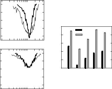
Figure 3.6A shows the typical pattern of a TTRS tuning curve. The heavy line is the threshold tuning curve, while TTRSa and TTRSb (the thin lines) depict the suppression threshold above and below the CF of the tuning curve. Figure 3.6B shows what happens shortly after removal from an intense sound exposure. As would be expected, the single tone tuning curve exhibits a threshold shift and broadening of tuning. The suppression slopes are shallower, the best suppression thresholds are elevated, and TTRSa and TTRSb are first identified at a frequency more distant from the CF than in the control (Fig. 3.6A). In addition, acoustic trauma reduced the number of neurons exhibiting these boundaries from 53% to 8% for TTRS below CF, and from 88% to 47% for boundaries above CF. The change in number of neurons showing TTRS boundaries in control and exposed animals, after different recovery intervals, appears in Figure 3.6C. The boundaries below CF have yet to fully recover after 28 days postexposure, while above CF, they returned to normal within 14 days. The incomplete recovery of the lower TTRS boundary has been related to the incompletely healed tectorial membrane in the overstimulated chicken ear.
3. Recovery of Function |
91 |
DECIBELS SPL
100 |
A |
|
|
|
|
|
80 |
|
|
|
|
|
|
60 |
|
TTRSb |
|
|
|
|
|
|
|
|
|
|
|
40 |
|
|
|
|
TTRSa |
|
|
Control |
|
|
|||
20 |
|
|
|
|
||
|
|
|
|
|
|
|
|
0.1 |
0.2 |
0.5 |
1.0 |
2.0 |
4.0 |
100 B
80
60
40
Exposed,
20 0-1D Recovered
0.10.2 0.5 1.0 2.0 4.0
FREQUENCY IN KHZ
PERCENT OF NEURONS
100 |
|
|
|
C |
TTRSb |
|
|
80 |
TTRSa |
|
|
|
|
|
|
60 |
|
|
|
|
|
||
40 |
|
||
|
|||
|
|
||
|
|
|
|
20 |
|
|
|
|
|
||
0 |
0-1D 5D 14D 28D |
||
Ctrl |
|||
|
CONDITIONS |
|
|
Figure 3.6. (A) A tuning curve from a nonexposed adult chicken cochlear nerve unit showing two-tone rate suppression boundaries above (TTRSa) and below (TTRSb) the unit CF. (B) A unit with a similar CF recorded shortly after removal from an intense sound exposure. The tuning curve is wider and CF threshold shows reduced sensitivity. The TTRS boundaries emerge at a much higher level along the skirts of the tuning curve. (C) The proportion of neurons in which TTRS revealed an upper or lower sideband in controls (Ctrl) or chickens allowed to recover 0–1, 5, 14, or 28 days. The suppression boundary above CF exhibits a normal incidence of occurrence 14 and 28 days postexposure, while suppression boundaries below CF never recover to normal. The asterisks indicate a significant difference from the control condition. (Data from Chen et al. 1997, with permission.)
2.3.5 Synchronization and Phase Locking
The ability of a cochlear nerve unit to discharge in concert with the cycles of a sinusoidal signal is referred to as synchronization. When synchronization occurs at a fixed phase angle, it is said to be “phase locked.” Figure 3.7A shows the phasic discharges in a peristimulus time (PST) histogram for a unit (CF = 0 42 kHz) stimulated repeatedly with a 0.42-kHz tone burst. The waveform of the tone burst is also plotted. The degree to which each cycle of the stimulus produces a phase-locked discharge can be used to calculate vector strength (VS) and the value of VS would equal one if every cycle of the stimulus produced a discharge. Inherent jitter at the hair cell synapse, limitations in the resistance/capacitance of the hair cell membrane, and limitiations in the influx