Diss / 3

Abstract—Direction-of-arrival estimation performance of MUSIC and maximum-likelihood estimation in the so-called “threshold” area is analyzed by means of general statistical analysis (GSA) (also known as random matrix theory). Both analytic predictions and direct Monte Carlo simulations demonstrate that the well-known MUSIC-specific “performance breakdown” is associated with the loss of resolution capability in the MUSIC pseudo-spectrum, while the sample signal subspace is still reliably separated from the actual noise subspace. Significant distinctions between (MUSIC/G-MUSIC)-specific and MLE-intrinsic causes of “performance breakdown,” as well as the role of “subspace swap” phenomena, are specified analytically and supported by simulation.

Index Terms—Array signal processing, generalized likelihoodratio tests, signal detection and estimation, G-estimation.

I. INTRODUCTION

I T has been known for a long time that when the sample support and/or signal-to-noise ratio (SNR) on an -variate antenna array is insufficient, MUSIC performance “breaks down” and rapidly departs from the CRB [1], [2]. In most studies, the phenomenon blamed for such performance breakdown in subspace-based methods is the so-called subspace swap when the “measured data is better approximated by some components of the orthogonal (“noise”) subspace than by the

components of the signal subspace” [3].

Analytical studies of this phenomenon usually rely upon the traditional asymptotic assumptions

and associated perturbation analysis of a sample covariance matrix eigendecomposition (see [4] for example). While max- imum-likelihood estimation (MLE) does not require signal eigenspace to be split into “signal” and “noise” subspaces, it has been known for a long time that under certain “threshold” conditions, MLE may also experience “performance breakdown” and generate severely erroneous estimates (“outliers”) not consistent with the CRB predictions (see [5, pp. 278–286]).

Manuscript received November 16, 2006; revised January 8, 2008. The associate editor coordinating the review of this manuscript and approving it for publication was Dr. Sven Nordebo. This work was funded under DSTO/RLM R&D Collaborative Agreement 290905.

B. A. Johnson is with RLM, Pty., Ltd., Edinburgh, SA, 5111, Australia, and also with the Institute for Telecommunications Research, University of South Australia, Mawson Lakes, SA, 5095 (e-mail: ben.a.johnson@ieee.org).

Y. I. Abramovich is with the Defence Science and Technology Organisation (DSTO), ISR Division, Edinburgh SA 5111, Australia (e-mail: yuri.abramovich@dsto.defence.gov.au).

X. Mestre is with the Centre Tecnològic de Telecomunicacions de Catalunya (CTTC), Castelldefels, 08860 Barcelona, Spain (e-mail: xavier.mestre@cttc. cat).

Digital Object Identifier 10.1109/TSP.2008.921729

Historically, analytical studies of MLE “breakdown” have been performed for a single signal in noise [6]–[9], or occasionally for multiple sources [10]–[12]), but almost always relying on traditional asymptotic perturbation analysis (with some notable exceptions, such as [13]). Since for a single source, MLE may be implemented via one-dimensional search (similar to MUSIC) over the traditional matched filter (beamformer) output, comparison with the MUSIC threshold condition is straightforward. For multiple sources, analysis of MLE threshold conditions is not as simple, primarily because the globally optimal ML solution often cannot be easily identified.

Yet, recent investigations for multiple source scenarios, conducted primarily by Monte Carlo simulations [14], demonstrated a “gap” in the minimum sample support and/or SNR between the MUSIC-specific and ML-intrinsic threshold conditions. In fact, it was demonstrated that for the considered multisource scenarios, MLE breakdown occurs at a significantly lower SNR than for MUSIC. It is therefore clear that for multiple-source scenarios, different mechanisms are responsible for MLE and MUSIC “breakdowns” which have not been thoroughly investigated.

In [15] and [16], an improvement in MUSIC “threshold performance” has been derived by X. Mestre, based on recent findings of the general statistical analysis (GSA) approach (also known as random matrix theory) that considers different asymptotic conditions

i.e., where both the array dimension and the number of snapshots grow without bound, but at the same rate.

While it was long known that for a finite , sample eigenvectors in the covariance matrix eigendecomposition

(2)

are biased estimates of the true eigenvectors , GSA methodology allowed Mestre to specify the ( consistent) G-MUSIC function such that (under certain conditions)

(3)

where is the MUSIC pseudospectrum of the true covariance matrix. Specifically

(4)

where is the -variate (unity norm) array steering vector in the direction and are the eigenvectors of the sample covariance matrix , associated with eigenvalues

. Note that for , the last eigenvalues are zero. For the known number of point sources, the G-weighting function , is [16]

(5)

with denoting the real valued solutions of

(6)

The weighting in (4) allows the parenthesized term to be treated as the consistent (under G-asymptotics) estimate of the noise subspace of the actual covariance matrix (where the subspace is an eigenvector matrix of the individual eigenvectors ).

While Mestre demonstrated some improvement in threshold conditions with respect to conventional MUSIC, he noted that “it was rather disappointing to observe that the use of -consistent estimates does not cure the breakdown effect of subspace-based techniques (in MUSIC) and it merely moves to a lower SNR” [17], indicating that G-MUSIC is not able to avoid the fundamental phenomena that separates MUSIC breakdown conditions from MLE ones. This was surprising given that the G-MUSIC derivations (3)–(6) and actual Monte Carlo simulations were conducted under conditions which “guarantee separation of the noise and first signal eigenvalue cluster of the asymptotic eigenvalue distribution of ” [15]. Therefore, G-asymptotically the “subspace swap” phenomenon is precluded by these conditions, and yet MUSIC and G-MUSIC breakdown was regularly observed in the conducted Monte Carlo trials under these conditions.

Clearly, the connections between “subspace swap” in MUSIC, G-MUSIC, and MLE “performance breakdown,” as well as the relevance of the GSA methodology for practically limited and values, needs to be clarified. In this paper, we introduce results of our attempts to do so. To this purpose, the paper is organized in a slightly unusual way, starting with simulation results and then examining some underlying theoretical considerations.

We start in Section II with the results of Monte Carlo trials for a typical multisource scenario that on one hand illustrates significantly better MLE performance in the “threshold” area compared with MUSIC and G-MUSIC, but more importantly serves as a test-case for GSA prediction accuracy assessment.

In Section III, we derive G-asymptotic “subspace swap” conditions and compare them with results of direct Monte Carlo trials. We demonstrate that for the considered scenarios, MUSIC-specific breakdown is associated with intersubspace “leakage” (rather than full subspace swap) whereby a small portion of the true signal eigenvector resides in the sample

noise subspace (and visa-versa). In Section IV, we show that this leakage is sufficient for loss of source resolution and associated MUSIC breakdown, and demonstrate a G-asymptotic prediction of the loss of resolution.

In Section V, we demonstrate that unlike MUSIC, the MLEintrinsic breakdown is directly associated with severe “subspace swap” in the sample covariance matrix, and therefore can be quite accurately predicted (in terms of SNR and sample support) for a given scenario. This is shown with both multisource and more traditional single source scenarios. In Section VI, we summarize and conclude the paper.

II. “PERFORMANCE BREAKDOWN” IN DOA ESTIMATION:

SIMULATION RESULTS

In this section, we illustrate MUSIC, G-MUSIC and MLE performance in the threshold region (of parameters) that spans the range from “proper” MUSIC behavior (no outliers) to MLE complete “performance breakdown.” For this reason, we once again consider the scenario used in [15], [18], and [19], with a -element uniform linear array (ULA), training samples, array element spacing of and independent equal power Gaussian sources (stochastic source model) located at azimuth angles

2010 35 37 (7)

immersed in white noise, with various per-element source SNRs (ranging from 15 to 25 dB, or set to specific SNRs for more detailed investigation).

The covariance matrix for this mixture is

(8)

where the noise power is ; source SNR is given by

, and is the DOA -dependent -variate “steering” (antenna manifold) vector.

The number of sources in our Monte Carlo simulations are assumed to be known a priori. MUSIC and G-MUSIC algorithms are implemented as usual by selecting the largest maxima of the MUSIC and G-MUSIC pseudo-spectra:

(9)

(10)

respectively, with as specified in (5)–(6).

In the Gaussian case, MLE is theoretically obtained by the selection of the single largest maxima of the multivariate likelihood function (LF) [20]

(11)

where represents the parameters power and angle of arrival for the sources. However, since the actual global extremum of the LF cannot be guaranteed in practice, MLE performance is assessed using an MLE-proxy algorithm [14]. The essence of this algorithm is to first find a local extremum of the likelihood function in the vicinity of the actual parameters for every Monte Carlo trial. We then make an initial “seed” estimate of the actual parameters using MUSIC or G-MUSIC to derive the DOAs and power estimation such as in [21]. This set of DOA estimates for a given trial is treated as representative of MLE performance if

(12)

In the event that the likelihood threshold is not exceeded, we use an iterative process to replace the MUSIC or G-MUSIC DOA estimates one by one with univariate LF searches. As opposed to approaches that are looking only for a local extremum in vicinity of the a priori known source location, this approach may initialize the ML search with a solution that is “far away” from the true one (when a “improper” MUSIC or G-MUSIC solution is used as the initial point). It is thus able to uncover “far away” maxima with a sufficient LF value to pass the threshold in (12) (i.e., MLE breakdown). If, however, the ML search results fail to meet the threshold condition (12) via whatever ML optimization approach we have chosen, then we treat this case as a failure of the optimization search routine to find a global maxima rather than an MLE failure and discard this result. Finally, the solutions are then evaluated for DOA estimation error. This ensures that, to the extent possible, even in the presence of MLE breakdown we are evaluating the underlying MLE performance.

While use of the threshold in (12) is not a practical approach, it adopts the same clairvoyant knowledge of the true solution as does the Cramér–Rao lower bound for MLE performance assessment. Also, while outside the scope of this paper, it should be noted that there are practical versions of this MLE-proxy algorithm [22], [23] which rely on statistical invariance of a modified likelihood ratio and have a quite reasonable threshold performance compared with the “clairvoyant” MLE-proxy algorithm used here.

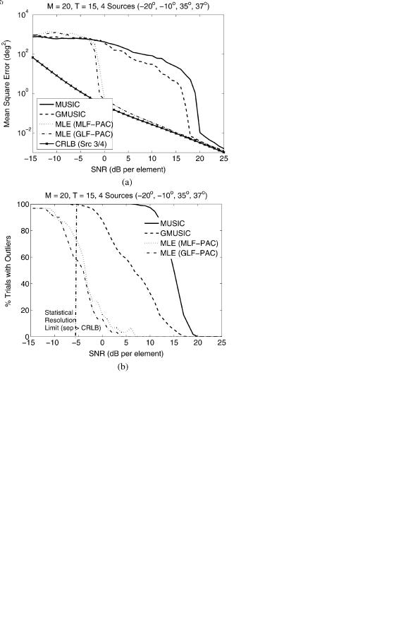
Fig. 1(a) shows the mean-square error (MSE), averaged over 300 trials, for DOA estimates of the two closely spaced sources (at 35 and 37 ). The figure demonstrates the familiar “threshold effect” in MSE for the DOA estimation process, with the sudden degradation in DOA accuracy (due to outliers) as the SNR is decreased. The MLE breakdown is demonstrated with the MLE-proxy algorithm discussed above, using two different “seeding” solutions produced by MUSIC and G-MUSIC correspondingly. Also shown is the stochastic Cramér-Rao bound (CRB) for the two sources at 35 and 37 (averaged together). One can observe the improvement in threshold performance delivered by G-MUSIC compared with MUSIC, as demonstrated in [15]. The improvement is more dramatic when examining the percentage of solutions that contain an outlier [Fig. 1(b)], as MUSIC deteriorates much more rapidly than G-MUSIC with decreasing SNR, but both algorithms are still outperformed by the MLE-proxy in this scenario.

Based on these introduced results, one has to conclude that for the considered multisource scenario, completely different

Fig. 1. Multiple-source estimation on a 20-element uniform linear array with training samples for MUSIC, G-MUSIC, and MLE. The SNR breakpoint (the “threshold”) decreases from around 20 dB for MUSIC to 17 dB for G-MUSIC, but is still dramatically greater than the MLE-proxy (LF-PAC) threshold observed at around 0 dB. Note that the invariance of the MLE-proxy results with respect to the “seeding” solution (MUSIC or G-MUSIC) indicates the reliable association of the results with true MLE performance in the threshold area. (a) Mean-square error. (b) Outlier production rate.

mechanisms drive (MUSIC/G-MUSIC)-specific and MLE-in- trinsic breakdown. This difference is the primary topic of our paper.

III. “SUBSPACE SWAP” AND MUSIC

“PERFORMANCE BREAKDOWN”

The subspace swap phenomenon has often been treated as the sole apparent mechanism “responsible” for performance breakdown in subspace-based techniques. This phenomenon is specified [3] as a case when the estimates of the noise subspace eigenvalues with increasing probability become larger than the estimates of the signal subspace eigenvalues . “More precisely, in such a case one or more pairs in the set actually estimate noise (subspace) eigenelements instead of signal elements,” Hawkes, Nehorai and Stoica note in [24]. The fact that subspace swap is associated with MUSIC breakdown has

order to simplify the analysis it is common practice to consider the particular case of the so-called “spiked population covariance matrix model.” This class of covariance matrix was introduced by Johnstone [27], and it describes the asymptotic behavior of a class of covariance matrices obtained from plane waves in noise (8). This model is essentially a particularization of the general one, based on the simplifying assumption that the contribution of the signal subspace is negligible in the asymptotic regime, in the sense that only the dimension of the noise subspace scales up with the number of antenna elements, whereas the dimension of the signal subspace remains fixed. Under this simplification of the original model (which implies letting for fixed in the above formulas), we see that the asymptotic subspace splitting condition in (16) becomes

(23)

or, equivalently, as

(29)

(30)

(31)

In addition, Paul also studied the convergence of the sample eigenvector when there is no asymptotic separation between signal and noise subspaces, namely . In particular, he established that, under the spiked population covariance matrix model

(36)

almost surely as at the same rate (in fact, Paul proved this for real-valued Gaussian observations with a diagonal covariance matrix, but we conjecture that the result is also valid for the observation model considered here).

In [28], Paul admitted that a “crucial aspect of the work [29], [30] is the discovery of a phase transition phenomenon,” which is clearly analogous to the subspace swap phenomena known in the signal processing literature for 20 years [31]. Here, we have shown that the condition (16), or the simplified one for the spiked population matrix (24), which asymptotically prevents the phase transition phenomenon from occurring, is in fact the condition which guarantees the separability of the signal and noise subspaces in the asymptotic sample eigenvalue distribution. Note that the subspace splitting condition (16) may be satisfied, preventing “inter-subspace” swap, while for some signal subspace eigenvalues, the similar eigenvalue splitting condition (14) may not be met. In that latter case, those sample signal subspace eigenvalues collapse into a single cluster, and the expressions (20)–(21) must be modified. Yet, this “intra-subspace” swap is not important for subspace techniques, where only intersubspace swap matters.

Tufts et al. [1] stated that the threshold effect was associated with the probability that the measured data is better approximated by some components of the orthogonal subspace than by some components of the signal subspace. A narrow investigation of the relationship between these G-asymptotic phase transitions and subspace swap would therefore pinpoint the conditions under which the norm of the scalar product between the true and estimated eigenvectors in the signal subspace fall below 0.5, in which case Tufts description of the subspace swap becomes clearly equivalent. Condition (24), obtained under the spiked population covariance model, implies that in our source scenario, when the eigenvalue is below the threshold , the projection of the fourth eigenvector onto the sample signal subspace

(37)

Furthermore, the “signal processing” subspace swap definition implies

(38)

or, equivalently

(39)

i.e., the last signal eigenvector is better represented by the noise subspace than the signal subspace. Therefore, the behavior of the projection is of prime importance for our analysis. In order to explore and validate these GSA analytic predictions with respect to MUSIC breakdown, let us analyze the

scenario (7) considered in Section II for the following four SNR values:

•Input SNR 25 dB no MUSIC outliers;

•Input SNR 14 dB 50% MUSIC outliers;

•Input SNR 9 dB almost100% MUSIC outliers;

•Input SNR 0 dB onset of ML breakdown.

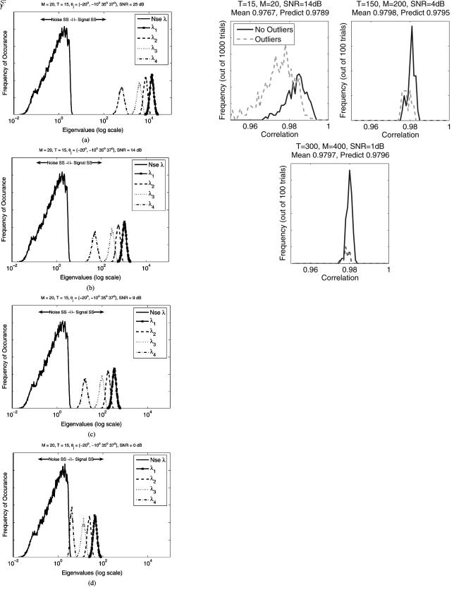
First, at Fig. 2 for each of these four SNR values we separately show the sample distributions of the four eigenvalues in the signal subspace, along with the distribution of all nonzero eigenvalues in the noise subspace. As expected, the separation between the noise and signal subspace eigenvalues decrease as the source SNR decreases, but one can see that even for the SNR of 9 dB with practically 100% MUSIC breakdown, the cluster of nonzero noise subspace eigenvalues is still well separated from the minimal signal subspace eigenvalue . It is only at the lowest plotted SNR of 0 dB that we see significant overlap between the noise and signal subspace eigenvalues. The eigenvalues for the underlying true covariance matrices (denoted Eig SNR are

which means that the subspace splitting condition from (24)

(44)

is satisfied for all four SNR values (although the 0 dB SNR case is marginal). The subspace splitting condition given in (16) can be computed for the transition from the signal subspace to the noise subspace which is the splitting condition between the 4th and 5th eigenvalues. This gives a value of 0.21, 0.24, 0.29, and 1.08 for 25, 14, 9, and 0 dB, respectively. This value is clearly less than for all but the last SNR value. Based on these GSA metrics only, one would conclude that the noise and signal subspace eigenvalues are distinct for all but the last case at 0 dB SNR, and therefore subspace techniques should operate robustly at the higher SNRs. Yet significant MUSIC breakdown occurs in the 9- and 14-dB SNR case. It is also important to establish that the finite conditions examined here do not change dramatically asymptotically (in the GSA sense (1)), so in addition to the scenario considered above, let us examine the following three scenarios with an increased and dimension, but with the ratio held constant.

The original scenario:

SNR 14 dB

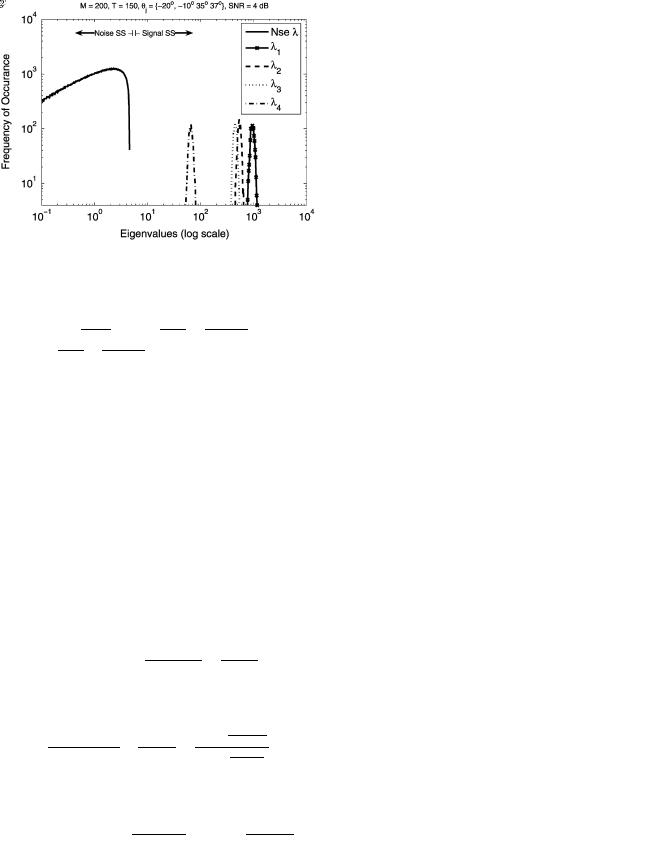
A 200-element array:

SNR 4 dB

Fig. 2. Eigenvalue Distributions for Scenario (7). Even in the presence of significant MUSIC breakdown for scenario SNR of 9 and 14 dB, the signal subspace eigenvalues remain well separated from the noise subspace eigenvalues.

(a) 25-dB SNR—No MUSIC Breakdown; (b) 14-dB SNR— 50% MUSIC outliers; (c) 9-dB SNR— 100 % MUSIC outliers; and (d) 0-dB SNR—Start of ML breakdown.

Fig. 3. Projection of 4th true eigenvector onto the sample signal subspace (scenario (45)–(47)). All scenarios show significant MUSIC breakdown ( 60 % 30 %, and 15 %, respectively), but the mean projection is converging to the predicted value in (56), whose high value indicates little subspace “leakage.”

A 400-element array with:

2010 35 35.1SNR 1 dB

Inter-source separations and SNR in the increased array size scenarios (46) and (47) have been chosen to produce essentially the same signal eigenvalues as per the original scenario (45) with . All three eigenspectra have minimal signal subspace eigenvalues in the range of 64–66, which would allow us to expect the same G-asymptotic behavior under the spiked population covariance model. At Fig. 3, we introduce sample distributions of the projection , calculated for all three scenarios (45), (46), (47) (with in all cases). First of all, we can clearly observe that in full agreement with GSA, the projection is converging as constant) to a non-statistical deterministic value. Indeed, one can observe quite a consistent convergence of the sample distributions for to a delta-function, whether the scenario contains a MUSIC outlier or not. Furthermore, while the results are converging asymptotically, the mean values observed at our modest array dimension of 20 elements are already quite accurate (to within 0.5% of the mean observed with 400 elements).

In order to predict these asymptotic deterministic values, let us consider the following Theorem 2 of Mestre [26].

JOHNSON et al.: MUSIC, G-MUSIC, AND ML PERFORMANCE BREAKDOWN

Theorem 2: If the splitting condition (16) for the smallest signal subspace eigenvalue is satisfied, the random value

(48)

where is a deterministic (unity norm) column vector, asymptotically tends to the nonrandom value , i.e.,

where

(50)

and are the eigenvectors of the matrix arranged in descending order and

(51)

where is the minimal (potentially negative) real-valued solution to

This theorem allows us to find the asymptotic MUSIC pseu-

where is specified by (51). Therefore, we get (for )

(54)

For the “spiked population covariance matrix”, when (27) (and ), we finally get

(55)

and for our specific scenario with the minimal signal subspace eigenvalue associated with

(56)

One can see that we get the same asymptotic expression as in (35), but now for the projection onto the entire sample subspace. This means that when the “intra-subspace swap” is precluded by

3951

Fig. 4. Eigenvalue distributions for first 4 eigenvalues and noise eigenvalues for scenario (46), SNR 4 dB. Note significant overlap between second and third eigenvalue distribution.

having the eigenvalue splitting condition (14) satisfied for all signal subspace eigenvectors, the power (35) of the true eigenvector asymptotically resides in the fourth sample subspace eigenvector , while the remaining power resides in the sample noise subspace. If instead only the subspace splitting condition (16) is satisfied , then the same power (56) is distributed across multiple sample signal subspace eigenvectors.

As can be observed in Fig. 3, the discrepancy between the estimated mean values for and the prediction (56) is within the fourth decimal point for a set of Monte Carlo trials and an array of elements. While the match for (56) is quite good even for small arrays, we separately observe that the projections of the sample eigenvectors onto the individual true signal subspace eigenvectors, can deviate significantly from (35) for even large arrays, under some circumstances. The problem occurs when the eigenvalue splitting condition (14) is not met for all signal subspace eigenvalues and “intra-subspace” swap within the signal subspace precludes individual projections from presenting values close to those predicted by (35). This difference between observation and prediction persists for large arrays if as grow, source separation is decreased, as we have done in (45)–(47). For the scenario (46) with elements, samples, and a very small difference between the second and third eigenvalue (see Fig. 4), intra-subspace swap for eigenvectors 2 and 3 was frequently observed with and the sample distribution of distributed widely over the [0 1] interval, as seen in Fig. 5. While this intra-subspace swap phenomena will not persist G-asymptotically as the relative dimension of the signal subspace vanishes, it still indicates that for breakdown analysis on finite arrays, the projection onto the entire subspace rather than individual eigenvectors is the appropriate metric.

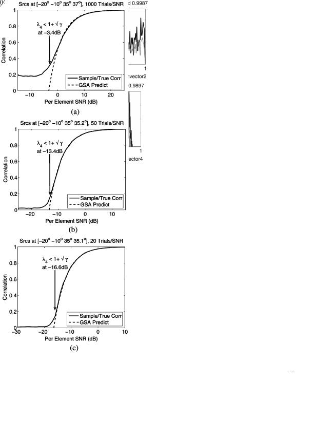
Finally, the most important observation from the MUSIC breakdown standpoint is that for both “proper” trials with no outliers and “improper” MUSIC trials with at least one outlier, the minimal signal subspace eigenvector still resides in the sample signal subspace with more than 95% of its power, converging asymptotically to 98%. This convergence is accurately

Fig. 5. Inner product of sample and true eigenvectors for element array and scenario (46). Correlation of the second and third sample eigenvectors with their associated true eigenvectors is poor because of frequent eigenvector swap, as is the match between the observed mean and the prediction from (35). Such “intra-subspace” swap should not affect MUSIC or any other subspace-based technique.

predicted by (56) for multiple SNR values, as indicated in Fig. 6.

The main conclusion that is now supported both by GSA theory and direct Monte Carlo simulations is that for the considered scenario, subspace swap is not responsible for the MUSIC breakdown phenomenon observed, and the underlying mechanism requires further exploration.

IV. SOURCE RESOLUTION AND MUSIC

“PERFORMANCE BREAKDOWN”

Careful examination of the pseudospectrum produced during trials with MUSIC outliers, such as in our scenario (7) with SNR dB, show that in many trials, the MUSIC algorithm selected an erroneous peak at despite the fact that the pseudo-spectrum value at that peak was significantly smaller than the pseudo-spectrum values at any true source direction

(57)

This happened only because MUSIC was unable to resolve the third and the fourth closely located sources 35 37 and instead found a single maxima in their vicinity. This well-known phenomena of loss of MUSIC resolution capability

[4] is not directly associated with the “subspace swap” phenomenon and in fact is associated with a significantly smaller portion of sample signal subspace energy residing in the noise subspace than is required for subspace swap as defined in (38). This fact has been already demonstrated by the experimental data in Figs. 3 –6 as well as the GSA prediction (56).

To examine the effect of this loss of resolution further, we need to define a “resolution event.” In [32], Cox defines a res-

Fig. 6. Comparison of predicted and observed projection of the fourth sample eigenvector onto the true signal subspace. The correspondence between the observations and the predictions above is accurate even at small array sizes such as the array. (a) ; (b)

; and (c) .

olution event for closely spaced sources, such as the DOAs and in scenario (7), as the event when

(58)

where . This condition means that the sample MUSIC pseudo-spectrum in the midpoint between the true DOAs ( and ) lies below the line that connects the pseudospectrum values at the true DOAs.