Wooldridge_-_Introductory_Econometrics_2nd_Ed

Appendix A Basic Mathematical Tools

PROPERTY SUM. 3: If {(xi,yi): i 1,2, …, n} is a set of n pairs of numbers, and a and b are constants, then

It is also important to be aware of some things that cannot be done with the summation operator. Let {(xi,yi): i 1,2, …, n} again be a set of n pairs of numbers with yi 0 for each i. Then,

In other words, the sum of the ratios is not the ratio of the sums. In the n 2 case, the application of familiar elementary algebra also reveals this lack of equality: x1/y1 x2/y2 (x1 x2)/(y1 y2). Similarly, the sum of the squares is not the square of the

ally equal is easiest to see when n 2: x21 x22 (x1 x2)2 x21 2x1x2 x22. Given n numbers {xi: i 1, …, n}, we compute their average or mean by adding

them up and dividing by n:

When the xi are a sample of data on a particular variable (such as years of education), we often call this the sample average (or sample mean) to emphasize that it is computed from a particular set of data. The sample average is an example of a descriptive statistic; in this case, the statistic describes the central tendency of the set of points xi.

There are some basic properties about averages that are important to understand. First, suppose we take each observation on x and subtract off the average: di xi x¯ (the “d ” here stands for deviation from the average). Then the sum of these deviations is always zero:

i 1

A simple numerical example shows how this works. Suppose n 5 and x1 6, x2 1, x3 2, x4 0, and x5 5. Then x¯ 2, and the demeaned sample is {4, 1, 4, 2,3}. Adding these up gives zero, which is just what equation (A.6) says.

In our treatment of regression analysis in Chapter 2, we need to know some additional algebraic facts involving deviations from sample averages. An important one is

644

that the sum of squared deviations is the sum of the squared xi minus n times the square of x¯:

This can be shown using basic properties of the summation operator:

nn

x2i 2x¯ xi n(x¯)2

Given a data set on two variables, {(xi,yi): i 1,2, …, n}, it can also be shown that

this is a generalization of equation (A.7) (there, yi xi for all i).

The average is the measure of central tendency that we will focus on in most of this text. However, it is sometimes informative to use the median (or sample median) to describe the central value. To obtain the median of the n numbers {x1, …, xn}, we first order the values of the xi from smallest to largest. Then, if n is odd, the sample median is the middle number of the ordered observations. For example, given the numbers { 4,8,2,0,21, 10,18}, the median value is 2 (since the ordered sequence is { 10, 4,0,2,8,18,21}). If we change the largest number in this list, 21, to twice its value, 42, the median is still 2. By contrast, the sample average would increase from 5 to 8, a sizable change. Generally, the median is less sensitive than the average to changes in the extreme values (large or small) in a list of numbers. This is why “median incomes” or “median housing values” are often reported, rather than averages, when summarizing income or housing values in a city or county.

If n is even, there is no unique way to define the median because there are two numbers at the center. Usually the median is defined to be the average of the two middle values (again, after ordering the numbers from smallest to largest). Using this rule, the median for the set of numbers {4,12,2,6} would be (4 6)/2 5.

A.2 PROPERTIES OF LINEAR FUNCTIONS

Linear functions play an important role in econometrics because they are simple to interpret and manipulate. If x and y are two variables related by

645

Appendix A Basic Mathematical Tools

then we say that y is a linear function of x, and 0 and 1 are two parameters (numbers) describing this relationship. The intercept is 0, and the slope is 1.

The defining feature of a linear function is that the change in y is always 1 times the change in x:

where denotes “change.” In other words, the marginal effect of x on y is constant and equal to 1.

E X A M P L E A . 1

( L i n e a r H o u s i n g E x p e n d i t u r e F u n c t i o n )

Suppose that the relationship between monthly housing expenditure and monthly income is

Then, for each additional dollar of income, 27 cents is spent on housing. If family income increases by $200, then housing expenditure increases by (.27)200 $54. This function is graphed in Figure A.1.

According to equation (A.11), a family with no income spends $164 on housing, which of course cannot be literally true. For low levels of income, this linear function would not describe the relationship between housing and income very well, which is why we will eventually have to use other types of functions to describe such relationships.

In (A.11), the marginal propensity to consume (MPC) housing out of income is .27. This is different from the average propensity to consume (APC), which is

housing

income 164/income .27.

The APC is not constant, it is always larger than the MPC, and it gets closer to the MPC as income increases.

Linear functions are easily defined for more than two variables. Suppose that y is related to two variables, x1 and x2, in the general form

It is rather difficult to envision this function because its graph is three-dimensional. Nevertheless, 0 is still the intercept (the value of y when x1 0 and x2 0), and 1 and 2 measure particular slopes. From (A.12), the change in y, for given changes in x1 and x2, is

646

Appendix A Basic Mathematical Tools

F i g u r e A . 1

Graph of housing 164 .27 income.

housing

164

If x2 does not change, that is, x2 0, then we have

y 1 x1 if x2 0,

so that 1 is the slope of the relationship in the direction of x1:

y

1 x1 if x2 0.

Because it measures how y changes with x1, holding x2 fixed, 1 is often called the partial effect of x1 on y. Since the partial effect involves holding other factors fixed, it is closely linked to the notion of ceteris paribus. The parameter 2 has a similar interpretation: 2 y/ x2 if x1 0, so that 2 is the partial effect of x2 on y.

E X A M P L E A . 2

( D e m a n d f o r C o m p a c t D i s c s )

For college students, suppose that the monthly quantity demanded of compact discs is related to the price of compact discs and monthly discretionary income by

647

Appendix A Basic Mathematical Tools

F i g u r e A . 2

Graph of quantity 120 9.8 price .03 income, with income fixed at $900.

quantity 147

quantity = –9.8 price

15 price

quantity 120 9.8 price .03 income,

where price is dollars per disk and income is measured in dollars. The demand curve is the relationship between quantity and price, holding income (and other factors) fixed. This is graphed in two dimensions in Figure A.2 at an income level of $900. The slope of the demand curve, 9.8, is the partial effect of price on quantity: holding income fixed, if the price of compact discs increases by one dollar, then the quantity demanded falls by 9.8. (We abstract from the fact that CDs can only be purchased in discrete units.) An increase in income simply shifts the demand curve up (changes the intercept), but the slope remains the same.

A.3 PROPORTIONS AND PERCENTAGES

Proportions and percentages play such an important role in applied economics that it is necessary to become very comfortable in working with them. Many quantities reported in the popular press are in the form of percentages; a few examples include interest rates, unemployment rates, and high school graduation rates.

648

An important skill is being able to convert between proportions and percentages. A percentage is easily obtained by multiplying a proportion by 100. For example, if the proportion of adults in a county with a high school degree is .82, then we say that 82% (82 percent) of adults have a high school degree. Another way to think of percents and proportions is that a proportion is the decimal form of a percent. For example, if the marginal tax rate for a family earning $30,000 per year is reported as 28%, then the proportion of the next dollar of income that is paid in income taxes is .28 (or 28 cents).

When using percentages, we often need to convert them to decimal form. For example, if a state sales tax is 6% and $200 is spent on a taxable item, then the sales tax paid is 200(.06) 12 dollars. If the annual return on a certificate of deposit (CD) is 7.6% and we invest $3,000 in such a CD at the beginning of the year, then our interest income is 3,000(.076) 228 dollars. As much as we would like it, the interest income is not obtained by multiplying 3,000 by 7.6.

We must be wary of proportions that are sometimes incorrectly reported as percentages in the popular media. If we read, “The percentage of high school students who drink alcohol is .57,” we know that this really means 57% (not just over one-half of a percent, as the statement literally implies). College volleyball fans are probably familiar with press clips containing statements such as “Her hitting percentage was .372.” This really means that her hitting percentage was 37.2%.

In econometrics, we are often interested in measuring the changes in various quantities. Let x denote some variable, such as an individual’s income, the number of crimes committed in a community, or the profits of a firm. Let x0 and x1 denote two values for x: x0 is the initial value, and x1 is the subsequent value. For example, x0 could be the annual income of an individual in 1994 and x1 the income of the same individual in 1995. The proportionate change in x in moving from x0 to x1 is simply

assuming, of course, that x0 0. In other words, to get the proportionate change, we simply divide the change in x by its initial value. This is a way of standardizing the change so that it is free of units. For example, if an individual’s income goes from $30,000 per year to $36,000 per year, then the proportionate change is 6,000/30,000

.20.

It is more common to state changes in terms of percentages. The percentage change in x in going from x0 to x1 is simply 100 times the proportionate change:

the notation “% x” is read as “the percentage change in x.” For example, when income goes from $30,000 to $33,750, income has increased by 12.5%; to get this, we simply multiply the proportionate change, .125, by 100.

Again, we must be on guard for proportionate changes that are reported as percentage changes. In the previous example, for instance, reporting the percentage change in income as .125 is incorrect and could lead to confusion.

When we look at changes in things like dollar amounts or population, there is no ambiguity about what is meant by a percentage change. By contrast, interpreting per-

649

centage change calculations can be tricky when the variable of interest is itself a percentage, something that happens often in economics and other social sciences. To illustrate, let x denote the percentage of adults in a particular city having a college education. Suppose the initial value is x0 24 (24% have a college education), and the new value is x1 30. There are two quantities we can compute to describe how the percentage of college-educated people has changed. The first is the change in x, x. In this case, x x1 x0 6: the percentage of people with a college education has increased by six percentage points. On the other hand, we can compute the percentage change in x using equation (A.15): % x 100[(30 24)/24] 25.

In this example, the percentage point change and the percentage change are very different. The percentage point change is just the change in the percentages. The percentage change is the change relative to the initial value. Generally, we must pay close attention to which number is being computed. The careful researcher makes this distinction perfectly clear; unfortunately, in the popular press as well as in academic research, the type of reported change is often unclear.

E X A M P L E A . 3

( M i c h i g a n S a l e s T a x I n c r e a s e )

In March 1994, Michigan voters approved a sales tax increase from 4% to 6%. In political advertisements, supporters of the measure referred to this as a two percentage point increase, or an increase of two cents on the dollar. Opponents to the tax increase called it a 50% increase in the sales tax rate. Both claims are correct; they are simply different ways of measuring the increase in the sales tax. Naturally, each group reported the measure that made their position most favorable.

For a variable such as salary, it makes no sense to talk of a “percentage point change in salary” because salary is not measured as a percentage. We can describe a change in salary either in dollar or percentage terms.

A.4 SOME SPECIAL FUNCTIONS AND THEIR PROPERTIES

In Section A.2, we reviewed the basic properties of linear functions. We already indicated one important feature of functions like y 0 1x: a one-unit change in x results in the same change in y, regardless of the initial value of x. As we noted earlier, this is the same as saying the marginal effect of x on y is constant, something that is not realistic for many economic relationships. For example, the important economic notion of diminishing marginal returns is not consistent with a linear relationship.

In order to model a variety of economic phenomena, we need to study several nonlinear functions. A nonlinear function is characterized by the fact that the change in y for a given change in x depends on the starting value of x. Certain nonlinear functions appear frequently in empirical economics, so it is important to know how to interpret them. A complete understanding of nonlinear functions takes us into the realm of cal-

650

culus. Here, we simply summarize the most significant aspects of the functions, leaving the details of some derivations for Section A.5.

Quadratic Functions

One simple way to capture diminishing returns is to add a quadratic term to a linear relationship. Consider the equation

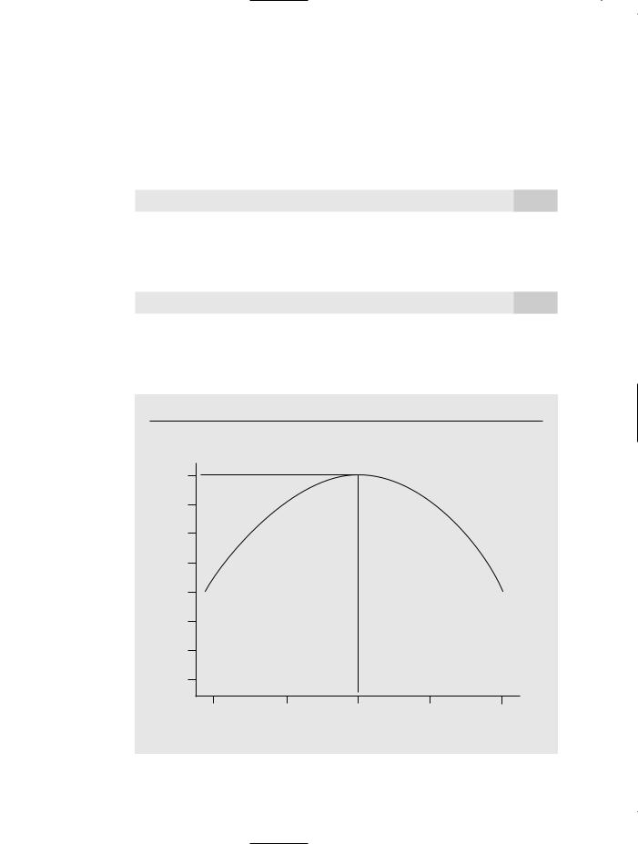
where 0, 1, and 2 are parameters. When 1 0 and 2 0, the relationship between y and x has the parabolic shape given in Figure A.3, where 0 6, 1 8, and 2 2.

When 1 0 and 2 0, it can be shown (using calculus in the next section) that

For example, if y 6 8x 2x2 (so 1 8, 2 2), then the largest value of y occurs at x* 8/4 2, and this value is 6 8(2) 2(2)2 14 (see Figure A.3).

F i g u r e A . 3

Graph of y 6 8x 2x2.

y

14

12

10

8

6

4

2

0

651

The fact that equation (A.16) implies a diminishing marginal effect of x on y is easily seen from its graph. Suppose we start at a low value of x and then increase x by some amount, say c. This has a larger effect on y than if we start at a higher value of x and increase x by the same amount c. In fact, once x x*, an increase in x actually decreases y.

The statement that x has a diminishing marginal effect on y is the same as saying that the slope of the function in Figure A.3 decreases as x increases. While this is clear from looking at the graph, we usually want to quantify how quickly the slope is changing. An application of calculus gives the approximate slope of the quadratic function as

for “small” changes in x. [The right-hand side of equation (A.18) is the derivative of the function in equation (A.16) with respect to x.] Another way to write this is

To see how well this approximation works, consider again the function y 6 8x 2x2. Then, according to equation (A.19), y (8 4x) x. Now, suppose we start at x 1 and change x by x .1. Using (A.19), y (8 4)(.1) .4. Of course, we can compute the change exactly by finding the values of y when x 1 and x 1.1: y0 6 8(1) 2(1)2 12 and y1 6 8(1.1) 2(1.1)2 12.38, and so the exact change in y is .38. The approximation is pretty close in this case.

Now, suppose we start at x 1 but change x by a larger amount: x .5. Then, the approximation gives y 4(.5) 2. The exact change is determined by finding the difference in y when x 1 and x 1.5. The former value of y was 12, and the latter value is 6 8(1.5) 2(1.5)2 13.5, so the actual change is 1.5 (not 2). The approximation is worse in this case because the change in x is larger.

For many applications, equation (A.19) can be used to compute the approximate marginal effect of x on y for any initial value of x and small changes. And, we can always compute the exact change if necessary.

E X A M P L E A . 4

( A Q u a d r a t i c W a g e F u n c t i o n )

Suppose the relationship between hourly wages and years in the work force (exper) is given by

This function has the same general shape as the one in Figure A.3. Using equation (A.17), exper has a positive effect on wage up to the turning point, exper* .48/[2(.008)] 30. The first year of experience is worth approximately .48, or 48 cents [see (A.19) with x 0, x 1]. Each additional year of experience increases wage by less than the previous

652

year—reflecting a diminishing marginal return to experience. At 30 years, an additional year of experience would actually lower the wage. This is not very realistic, but it is one of the consequences of using a quadratic function to capture a diminishing marginal effect: at some point, the function must reach a maximum and curve downward. For practical purposes, the point at which this happens is often large enough to be inconsequential, but not always.

The graph of the quadratic function in (A.16) has a U-shape if 1 0 and 2 0, in which case there is an increasing marginal return. The minimum of the function is at the point 1/(2 2).

The Natural Logarithm

The nonlinear function that plays the most important role in econometric analysis is the natural logarithm. In this text, we denote the natural logarithm, which we often refer to simply as the log function, as

You might remember learning different symbols for the natural log; ln(x) or loge(x) are the most common. These different notations are useful when logarithms with several different bases are being used. For our purposes, only the natural logarithm is important, and so log(x) denotes the natural logarithm throughout this text. This corresponds to the notation usage in many statistical packages, although some use ln(x) [and most calculators use ln(x)]. Economists use both log(x) and ln(x), which is useful to know when you are reading papers in applied economics.

The function y log(x) is defined only for x 0, and it is plotted in Figure A.4. It is not very important to know how the values of log(x) are obtained. For our purposes,

Several things are apparent from Figure A.4. First, when y log(x), the relationship between y and x displays diminishing marginal returns. One important difference between the log and the quadratic function in Figure A.3 is that when y log(x), the effect of x on y never becomes negative: the slope of the function gets closer and closer to zero as x gets large, but the slope never quite reaches zero and certainly never becomes negative.

The following are also apparent from Figure A.4:

log(x) 0 for 0 x 1 log(1) 0

log(x) 0 for x 1.

In particular, log(x) can be positive or negative. Some useful algebraic facts about the log function are

653