Wooldridge_-_Introductory_Econometrics_2nd_Ed

Part 2 Regression Analysis with Time Series Data

where oldindexnewbase is the original value of the index in the new base year. For example, with base year 1987, the IIP in 1992 is 107.7; if we change the base year to 1982,

the IIP in 1992 becomes 100(107.7/81.9) 131.5 (because the IIP in 1982 was 81.9). Another important example of an index number is a price index, such as the consumer price index (CPI). We already used the CPI to compute annual inflation rates in Example 10.1. As with the industrial production index, the CPI is only meaningful when we compare it across different years (or months, if we are using monthly data). In the 1997 ERP, CPI 38.8 in 1970, and CPI 130.7 in 1990. Thus, the general price level grew by almost 237% over this twenty-year period. (In 1997, the CPI is defined so that its average

in 1982, 1983, and 1984 equals 100; thus, the base period is listed as 1982–1984.)

In addition to being used to compute inflation rates, price indexes are necessary for turning a time series measured in nominal dollars (or current dollars) into real dollars

(or constant dollars). Most economic behavior is assumed to be influenced by real, not nominal, variables. For example, classical labor economics assumes that labor supply is based on the real hourly wage, not the nominal wage. Obtaining the real wage from the nominal wage is easy if we have a price index such as the CPI. We must be a little careful to first divide the CPI by 100, so that the value in the base year is one. Then, if w denotes the average hourly wage in nominal dollars and p CPI/100, the real wage is simply w/p. This wage is measured in dollars for the base period of the CPI. For example, in Table B-45 in the 1997 ERP, average hourly earnings are reported in nominal terms and in 1982 dollars (which means that the CPI used in computing the real wage had the base year 1982). This table reports that the nominal hourly wage in 1960 was $2.09, but measured in 1982 dollars, the wage was $6.79. The real hourly wage had peaked in 1973, at $8.55 in 1982 dollars, and had fallen to $7.40 by 1995. Thus, there has been a nontrivial decline in real wages over the past 20 years. (If we compare nominal wages from 1973 and 1995, we get a very misleading picture: $3.94 in 1973 and $11.44 in 1995. Since the real wage has actually fallen, the increase in the nominal wage is due entirely to inflation.)

Standard measures of economic output are in real terms. The most important of these is gross domestic product, or GDP. When growth in GDP is reported in the popular press, it is always real GDP growth. In the 1997 ERP, Table B-9, GDP is reported in billions of 1992 dollars. We used a similar measure of output, real gross national product, in Example 10.3.

Interesting things happen when real dollar variables are used in combination with natural logarithms. Suppose, for example, that average weekly hours worked are related to the real wage as

log(hours) 0 1log(w/p) u.

Using the fact that log(w/p) log(w) log(p), we can write this as

but with the restriction that 2 1. Therefore, the assumption that only the real wage influences labor supply imposes a restriction on the parameters of model (10.21).

328

If 2 1, then the price level has an effect on labor supply, something that can happen if workers do not fully understand the distinction between real and nominal wages.

There are many practical aspects to the actual computation of index numbers, but it would take us too far afield to cover those here. Detailed discussions of price indexes can be found in most intermediate macroeconomic texts, such as Mankiw (1994, Chapter 2). For us, it is important to be able to use index numbers in regression analysis. As mentioned earlier, since the magnitudes of index numbers are not especially informative, they often appear in logarithmic form, so that regression coefficients have percentage change interpretations.

We now give an example of an event study that also uses index numbers.

E X A M P L E 1 0 . 5

( A n t i d u m p i n g F i l i n g s a n d C h e m i c a l I m p o r t s )

Krupp and Pollard (1996) analyzed the effects of antidumping filings by U.S. chemical industries on imports of various chemicals. We focus here on one industrial chemical, barium chloride, a cleaning agent used in various chemical processes and in gasoline production. In the early 1980s, U.S. barium chloride producers believed that China was offering its U.S. imports at an unfairly low price (an action known as dumping), and the barium chloride industry filed a complaint with the U.S. International Trade Commission (ITC) in October 1983. The ITC ruled in favor of the U.S. barium chloride industry in October 1984. There are several questions of interest in this case, but we will touch on only a few of them. First, are imports unusually high in the period immediately preceding the initial filing? Second, do imports change noticeably after an antidumping filing? Finally, what is the reduction in imports after a decision in favor of the U.S. industry?

To answer these questions, we follow Krupp and Pollard by defining three dummy variables: befile6 is equal to one during the six months before filing, affile6 indicates the six months after filing, and afdec6 denotes the six months after the positive decision. The dependent variable is the volume of imports of barium chloride from China, chnimp, which we use in logarithmic form. We include as explanatory variables, all in logarithmic form, an index of chemical production, chempi (to control for overall demand for barium chloride), the volume of gasoline production, gas (another demand variable), and an exchange rate index, rtwex, which measures the strength of the dollar against several other currencies. The chemical production index was defined to be 100 in June 1977. The analysis here differs somewhat from Krupp and Pollard in that we use natural logarithms of all variables (except the dummy variables, of course), and we include all three dummy variables in the same regression.

Using monthly data from February 1978 through December 1988 gives the following:

329

The equation shows that befile6 is statistically insignificant, so there is no evidence that Chinese imports were unusually high during the six months before the suit was filed. Further, although the estimate on affile6 is negative, the coefficient is small (indicating about a 3.2% fall in Chinese imports), and it is statistically very insignificant. The coefficient on afdec6 shows a substantial fall in Chinese imports of barium chloride after the decision in favor of the U.S. industry, which is not surprising. Since the effect is so large, we compute the exact percentage change: 100[exp( .566) 1] 43.2%. The coefficient is statistically significant at the 5% level against a two-sided alternative.

The coefficient signs on the control variables are what we expect: an increase in overall chemical production increases the demand for the cleaning agent. Gasoline production does not affect Chinese imports significantly. The coefficient on log(rtwex) shows that an increase in the value of the dollar relative to other currencies increases the demand for Chinese imports, as is predicted by economic theory. (In fact, the elasticity is not statistically different from one. Why?)

Interactions among qualitative and quantitative variables are also used in time series analysis. An example with practical importance follows.

E X A M P L E 1 0 . 6

( E l e c t i o n O u t c o m e s a n d E c o n o m i c P e r f o r m a n c e )

Fair (1996) summarizes his work on explaining presidential election outcomes in terms of economic performance. He explains the proportion of the two-party vote going to the Democratic candidate using data for the years 1916 through 1992 (every four years) for a total of 20 observations. We estimate a simplified version of Fair’s model (using variable names that are more descriptive than his):

demvote 0 1 partyWH 2incum 3partyWH gnews4 partyWH inf u,

where demvote is the proportion of the two-party vote going to the Democratic candidate. The explanatory variable partyWH is similar to a dummy variable, but it takes on the value one if a Democrat is in the White House and 1 if a Republican is in the White House. Fair uses this variable to impose the restriction that the effect of a Republican being in the White House has the same magnitude but opposite sign as a Democrat being in the White House. This is a natural restriction since the party shares must sum to one, by definition. It also saves two degrees of freedom, which is important with so few observations. Similarly, the variable incum is defined to be one if a Democratic incumbent is running, 1 if a Republican incumbent is running, and zero otherwise. The variable gnews is the number of quarters during the current administration’s first 15 (out of 16 total), where the quarterly growth in real per capita output was above 2.9% (at an annual rate), and inf is the average annual inflation rate over the first 15 quarters of the administration. See Fair (1996) for precise definitions.

Economists are most interested in the interaction terms partyWH gnews and partyWH inf. Since partyWH equals one when a Democrat is in the White House, 3 measures the effect of good economic news on the party in power; we expect 3 0. Similarly,

330

4 measures the effect that inflation has on the party in power. Because inflation during an administration is considered to be bad news, we expect 4 0.

The estimated equation using the data in FAIR.RAW is

All coefficients, except that on partyWH, are statistically significant at the 5% level. Incumbency is worth about 5.4 percentage points in the share of the vote. (Remember, demvote is measured as a proportion.) Further, the economic news variable has a positive effect: one more quarter of good news is worth about 1.1 percentage points. Inflation, as expected, has a negative effect: if average annual inflation is, say, two percentage points higher, the party in power loses about 1.5 percentage points of the two-party vote.

We could have used this equation to predict the outcome of the 1996 presidential election between Bill Clinton, the Democrat, and Bob Dole, the Republican. (The independent candidate, Ross Perot, is excluded because Fair’s equation is for the two-party vote only.) Since Clinton ran as an incumbent, partyWH 1 and incum 1. To predict the election outcome, we need the variables gnews and inf. During Clinton’s first 15 quarters in office, per capita real GDP exceeded 2.9% three times, so gnews 3. Further, using the GDP price deflator reported in Table B-4 in the 1997 ERP, the average annual inflation rate (computed using Fair’s formula) from the fourth quarter in 1991 to the third quarter in 1996 was 3.019. Plugging these into (10.23) gives

Therefore, based on information known before the election in November, Clinton was predicted to receive a very slight majority of the two-party vote: about 50.1%. In fact, Clinton won more handily: his share of the two-party vote was 54.65%.

10.5 TRENDS AND SEASONALITY

Characterizing Trending Time Series

Many economic time series have a common tendency of growing over time. We must recognize that some series contain a time trend in order to draw causal inference using time series data. Ignoring the fact that two sequences are trending in the same or opposite directions can lead us to falsely conclude that changes in one variable are actually caused by changes in another variable. In many cases, two time series processes appear to be correlated only because they are both trending over time for reasons related to other unobserved factors.

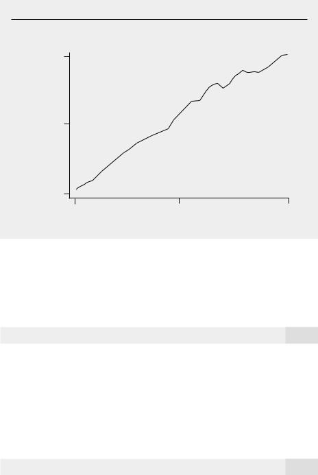
Figure 10.2 contains a plot of labor productivity (output per hour of work) in the United States for the years 1947 through 1987. This series displays a clear upward trend, which reflects the fact that workers have become more productive over time.

331

Part 2 Regression Analysis with Time Series Data

F i g u r e 1 0 . 2

Output per labor hour in the United States during the years 1947–1987; 1977 100.

output 110 per

hour

80

50

Other series, at least over certain time periods, have clear downward trends. Because positive trends are more common, we will focus on those during our discussion.

What kind of statistical models adequately capture trending behavior? One popular formulation is to write the series {yt} as

where, in the simplest case, {et} is an independent, identically distributed (i.i.d.) sequence with E(et) 0, Var(et) 2e. Note how the parameter 1 multiplies time, t, resulting in a linear time trend. Interpreting 1 in (10.24) is simple: holding all other factors (those in et) fixed, 1 measures the change in yt from one period to the next due to the passage of time: when et 0,

yt yt yt 1 1.

Another way to think about a sequence that has a linear time trend is that its average value is a linear function of time:

If 1 0, then, on average, yt is growing over time and therefore has an upward trend. If 1 0, then yt has a downward trend. The values of yt do not fall exactly on the line

332

Chapter 10 Basic Regression Analysis with Time Series Data

characterization of trending time series allows {et} to be correlated over time, but this does not change the flavor of a linear time trend. In fact, what is important for regression analysis under the classical linear model assumptions is that E(yt) is linear in t. When we cover large sample properties of OLS in Chapter 11, we will have to discuss how much temporal correlation in {et} is allowed.

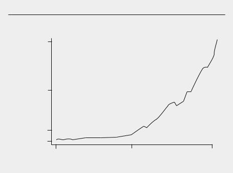
Many economic time series are better approximated by an exponential trend, which follows when a series has the same average growth rate from period to period. Figure 10.3 plots data on annual nominal imports for the United States during the years 1948 through 1995 (ERP 1997, Table B–101).

In the early years, we see that the change in the imports over each year is relatively small, whereas the change increases as time passes. This is consistent with a constant average growth rate: the percentage change is roughly the same in each period.

In practice, an exponential trend in a time series is captured by modeling the natural logarithm of the series as a linear trend (assuming that yt 0):

F i g u r e 1 0 . 3

Nominal U.S. imports during the years 1948–1995 (in billions of U.S. dollars).

U.S. 750 imports

400

100

7

333

Part 2 Regression Analysis with Time Series Data

Exponentiating shows that yt itself has an exponential trend: yt exp( 0 1t et). Because we will want to use exponentially trending time series in linear regression models, (10.26) turns out to be the most convenient way for representing such series.

How do we interpret 1 in (10.26)? Remember that, for small changes, log(yt) log(yt) log(yt 1) is approximately the proportionate change in yt:

The right-hand side of (10.27) is also called the growth rate in y from period t 1 to period t. To turn the growth rate into a percent, we simply multiply by 100. If yt follows (10.26), then, taking changes and setting et 0,

In other words, 1 is approximately the average per period growth rate in yt. For example, if t denotes year and 1 .027, then yt grows about 2.7% per year on average.

Although linear and exponential trends are the most common, time trends can be more complicated. For example, instead of the linear trend model in (10.24), we might have a quadratic time trend:

If 1 and 2 are positive, then the slope of the trend is increasing, as is easily seen by computing the approximate slope (holding et fixed):

[If you are familiar with calculus, you recognize the right-hand side of (10.30) as the derivative of 0 1t 2t 2 with respect to t.] If 1 0, but 2 0, the trend has a hump shape. This may not be a very good description of certain trending series because it requires an increasing trend to be followed, eventually, by a decreasing trend. Nevertheless, over a given time span, it can be a flexible way of modeling time series that have more complicated trends than either (10.24) or (10.26).

Using Trending Variables in Regression Analysis

Accounting for explained or explanatory variables that are trending is fairly straightforward in regression analysis. First, nothing about trending variables necessarily violates the classical linear model assumptions, TS.1 through TS.6. However, we must be careful to allow for the fact that unobserved, trending factors that affect yt might also be correlated with the explanatory variables. If we ignore this possibility, we may find a spurious relationship between yt and one or more explanatory variables. The phenomenon of finding a relationship between two or more trending variables simply

334

because each is growing over time is an example of spurious regression. Fortunately, adding a time trend eliminates this problem.

For concreteness, consider a model where two observed factors, xt1 and xt2, affect yt. In addition, there are unobserved factors that are systematically growing or shrinking over time. A model that captures this is

This fits into the multiple linear regression framework with xt3 t. Allowing for the trend in this equation explicitly recognizes that yt may be growing ( 3 0) or shrinking ( 3 0) over time for reasons essentially unrelated to xt1 and xt2. If (10.31) satisfies assumptions TS.1, TS.2, and TS.3, then omitting t from the regression and regressing yt on xt1, xt2 will generally yield biased estimators of 1 and 2: we have effectively omitted an important variable, t, from the regression. This is especially true if xt1 and xt2 are themselves trending, because they can then be highly correlated with t. The next example shows how omitting a time trend can result in spurious regression.

E X A M P L E 1 0 . 7

( H o u s i n g I n v e s t m e n t a n d P r i c e s )

The data in HSEINV.RAW are annual observations on housing investment and a housing price index in the United States for 1947 through 1988. Let invpc denote real per capita housing investment (in thousands of dollars) and let price denote a housing price index (equal to one in 1982). A simple regression in constant elasticity form, which can be thought of as a supply equation for housing stock, gives

The elasticity of per capita investment with respect to price is very large and statistically significant; it is not statistically different from one. We must be careful here. Both invpc and price have upward trends. In particular, if we regress log(invpc) on t, we obtain a coefficient on the trend equal to .0081 (standard error .0018); the regression of log(price) on t yields a trend coefficient equal to .0044 (standard error .0004). While the standard errors on the trend coefficients are not necessarily reliable—these regressions tend to contain substantial serial correlation—the coefficient estimates do reveal upward trends.

To account for the trending behavior of the variables, we add a time trend:

The story is much different now: the estimated price elasticity is negative and not statistically different from zero. The time trend is statistically significant, and its coefficient implies

335

an approximate 1% increase in invpc per year, on average. From this analysis, we cannot conclude that real per capita housing investment is influenced at all by price. There are other factors, captured in the time trend, that affect invpc, but we have not modeled these. The results in (10.32) show a spurious relationship between invpc and price due to the fact that price is also trending upward over time.

In some cases, adding a time trend can make a key explanatory variable more significant. This can happen if the dependent and independent variables have different kinds of trends (say, one upward and one downward), but movement in the independent variable about its trend line causes movement in the dependent variable away from its trend line.

E X A M P L E 1 0 . 8

( F e r t i l i t y E q u a t i o n )

If we add a linear time trend to the fertility equation (10.18), we obtain

The coefficient on pe is more than triple the estimate from (10.18), and it is much more statistically significant. Interestingly, pill is not significant once an allowance is made for a linear trend. As can be seen by the estimate, gfr was falling, on average, over this period, other factors being equal.

Since the general fertility rate exhibited both upward and downward trends during the period from 1913 through 1984, we can see how robust the estimated effect of pe is when we use a quadratic trend:

The coefficient on pe is even larger and more statistically significant. Now, pill has the expected negative effect and is marginally significant, and both trend terms are statistically significant. The quadratic trend is a flexible way to account for the unusual trending behavior of gfr.

You might be wondering in Example 10.8: Why stop at a quadratic trend? Nothing prevents us from adding, say, t3 as an independent variable, and, in fact, this might be

336

warranted (see Exercise 10.12). But we have to be careful not to get carried away when including trend terms in a model. We want relatively simple trends that capture broad movements in the dependent variable that are not explained by the independent variables in the model. If we include enough polynomial terms in t, then we can track any series pretty well. But this offers little help in finding which explanatory variables affect yt.

A Detrending Interpretation of Regressions with a Time Trend

Including a time trend in a regression model creates a nice interpretation in terms of detrending the original data series before using them in regression analysis. For concreteness, we focus on model (10.31), but our conclusions are much more general.

When we regress yt on xt1, xt2 and t, we obtain the fitted equation

We can extend the results on the partialling out interpretation of OLS that we covered in Chapter 3 to show that ˆ1 and ˆ2 can be obtained as follows.

(i) Regress each of yt, xt1 and xt2 on a constant and the time trend t and save the residuals, say yt, xt1, xt2, t 1,2, …, n. For example,

yt yt ˆ0 ˆ1t.

Thus, we can think of yt as being linearly detrended. In detrending yt, we have estimated the model

yt 0 1t et

by OLS; the residuals from this regression, eˆt yt, have the time trend removed (at least in the sample). A similar interpretation holds for xt1 and xt2.

(ii) Run the regression of

(No intercept is necessary, but including an intercept affects nothing: the intercept will be estimated to be zero.) This regression exactly yields ˆ1 and ˆ2 from (10.36).

This means that the estimates of primary interest, ˆ1 and ˆ2, can be interpreted as coming from a regression without a time trend, but where we first detrend the dependent variable and all other independent variables. The same conclusion holds with any number of independent variables and if the trend is quadratic or of some other polynomial degree.

If t is omitted from (10.36), then no detrending occurs, and yt might seem to be related to one or more of the xtj simply because each contains a trend; we saw this in Example 10.7. If the trend term is statistically significant, and the results change in important ways when a time trend is added to a regression, then the initial results without a trend should be treated with suspicion.

The interpretation of ˆ1 and ˆ2 shows that it is a good idea to include a trend in the regression if any independent variable is trending, even if yt is not. If yt has no noticeable trend, but, say, xt1 is growing over time, then excluding a trend from the regression

337