

6Point Location
Knowing Where You Are
This book has, for the most part, been written in Europe. More precisely, it has been written very close to a point at longitude 5◦6 east and latitude 52◦3 north. Where that is? You can find that out yourself from a map of Europe: using the scales on the sides of the map, you will find that the point with the coordinates stated above is located in a little country named “the Netherlands”.
In this way you would have answered a point location query: Given a map and a query point q specified by its coordinates, find the region of the map containing q. A map, of course, is nothing more than a subdivision of the plane into regions, a planar subdivision, as defined in Chapter 2.
5◦6
52◦3
Figure 6.1
Point location in a map
Point location queries arise in various settings. Suppose that you are sailing on |
|
a sea with sand banks and dangerous currents in various parts of it. To be able |
|
to navigate safely, you will have to know the current at your present position. |
|
Fortunately there are maps that indicate the kind of current in the various parts |
|
of the sea. To use such a map, you will have to do the following. First, you must |
|
determine your position. Until not so long ago, you would have to rely for this |
121 |
Chapter 6
POINT LOCATION
on the stars or the sun, and a good chronometer. Nowadays it is much easier to determine your position: there are little boxes on the market that compute your position for you, using information from various satellites. Once you have determined the coordinates of your position, you will have to locate the point on the map showing the currents, or to find the region of the sea you are presently in.
One step further would be to automate this last step: store the map electronically, and let the computer do the point location for you. It could then display the current—or any other information for which you have a thematic map in electronic form—of the region you are in continuously. In this situation we have a set of presumably rather detailed thematic maps and we want to answer point location queries frequently, to update the displayed information while the ship is moving. This means that we will want to preprocess the maps, and to store them in a data structure that makes it possible to answer point location queries fast.
Point location problems arise on a quite different scale as well. Assume that we want to implement an interactive geographic information system that displays a map on a screen. By clicking with the mouse on a country, the user can retrieve information about that country. While the mouse is moved the system should display the name of the country underneath the mouse pointer somewhere on the screen. Every time the mouse is moved, the system has to recompute which name to display. Clearly this is a point location problem in the map displayed on the screen, with the mouse position as the query point. These queries occur with high frequency—after all, we want to update the screen information in real time—and therefore have to be answered fast. Again, we need a data structure that supports fast point location queries.
|
|
|
|
6.1 Point Location and Trapezoidal Maps |
|
|
|
|
Let S be a planar subdivision with n edges. The planar point location problem |
|
|
|
|
is to store S in such a way that we can answer queries of the following type: |
|
|
|
|
Given a query point q, report the face f of S that contains q. If q lies on an edge |
|
|
|
|
or coincides with a vertex, the query algorithm should return this information. |
|
|
|
||
|
|
|
|
To get some insight into the problem, let’s first give a very simple data structure |
|
|
|
|
to perform point location queries. We draw vertical lines through all vertices of |
|
|
|
|
the subdivision, as in Figure 6.2. This partitions the plane into vertical slabs. |
|
|
|
|
We store the x-coordinates of the vertices in sorted order in an array. This |
|
|
|
|
makes it possible to determine in O(log n) time the slab that contains a query |
|
|
|
|
point q. Within a slab, there are no vertices of S. This means that the part of the |
|
|
|
|
subdivision lying inside the slab has a special form: all edges intersecting a slab |
|
|
|
|
completely cross it—they have no endpoint in the slab—and they don’t cross |
|
|
|
|
each other. This means that they can be ordered from top to bottom. Notice |
|
|
|
||
|
|
|
|
that every region in the slab between two consecutive edges belongs to a unique |
122 |
|
|
|
face of S. The lowest and highest region of the slab are unbounded, and are part |
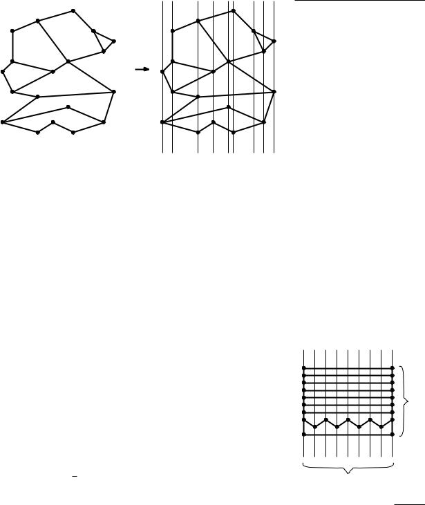
of the unbounded face of S. The special structure of the edges intersecting a slab implies that we can store them in sorted order in an array. We label each edge with the face of S that is immediately above it inside the slab.
The total query algorithm is now as follows. First, we do a binary search with the x-coordinate of the query point q in the array storing the x-coordinates of the vertices of the subdivision. This tells us the slab containing q. Then we do a binary search with q in the array for that slab. The elementary operation in this binary search is: Given a segment s and a point q such that the vertical line through q intersects s, determine whether q lies above s, below s, or on s. This tells us the segment directly below q, provided there is one. The label stored with that segment is the face of S containing q. If we find that there is no segment below q then q lies in the unbounded face.
The query time for the data structure is good: we only perform two binary searches, the first in an array of length at most 2n (the n edges of the subdivision have at most 2n vertices), and the second in an array of length at most n (a slab is crossed by at most n edges). Hence, the query time is O(log n).
What about the storage requirements? First of all, we have an array on the x-coordinates of the vertices, which uses O(n) storage. But we also have an array for every slab. Such an array stores the edges intersecting its slab, so it uses O(n) storage. Since there are O(n) slabs, the total amount of storage is O(n2). It’s easy to give an example where n/4 slabs are intersected by n/4 edges each, which shows that this worst-case bound can actually occur.
The amount of storage required makes this data structure rather uninteresting— a quadratic size structure is useless in most practical applications, even for moderately large values of n. (One may argue that in practice the quadratic behavior does not occur. But it is rather likely that the amount of storage is something like O(n√n).) Where does this quadratic behavior come from? Let’s have a second look at Figure 6.2. The segments and the vertical lines through the endpoints define a new subdivision S , whose faces are trapezoids, triangles, and unbounded trapezoid-like faces. Furthermore, S is a refinement of the original
Section 6.1
POINT LOCATION AND TRAPEZOIDAL
MAPS
Figure 6.2
Partition into slabs
n
4
n4 slabs
123
Chapter 6
POINT LOCATION
124
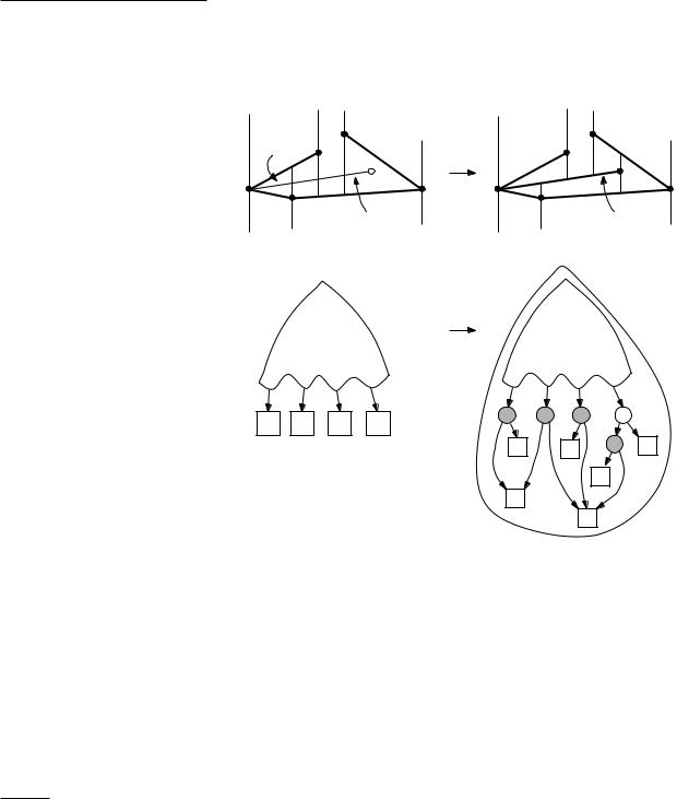
subdivision S: every face of S lies completely in one face of S. The query algorithm described above is in fact an algorithm to do planar point location in this refined subdivision. This solves the original planar point location as well: because S is a refinement of S, once we know the face f S containing q, we know the face f S containing q. Unfortunately, the refined subdivision can have quadratic complexity. It is therefore not surprising that the resulting data structure has quadratic size.
Perhaps we should look for a different refinement of S that—like the decomposition shown above—makes point location queries easier, and that—unlike the decomposition shown above—has a complexity that is not much larger than the complexity of the original subdivision S. Indeed such a refinement exists. In the rest of this section, we shall describe the trapezoidal map, a refinement that has the desirable properties just mentioned.
We call two line segments in the plane non-crossing if their intersection is either empty or a common endpoint. Notice that the edges of any planar subdivision are non-crossing.
Let S be a set of n non-crossing segments in the plane. Trapezoidal maps can be defined for such sets in general, but we shall make two simplifications that make life easier for us in this and the next sections.
First, it will be convenient to get rid of the unbounded trapezoid-like faces that occur at the boundary of the scene. This can be done by introducing a large, axis-parallel rectangle R that contains the whole scene, that is, that contains all segments of S. For our application—point location in subdivisions—this is not a problem: a query point outside R always lies in the unbounded face of S, so we can safely restrict our attention to what happens inside R.
The second simplification is more difficult to justify: we will assume that no two distinct endpoints of segments in the set S have the same x-coordinate. A consequence of this is that there cannot be any vertical segments. This assumption is not very realistic: vertical edges occur frequently in many applications, and the situation that two non-intersecting segments have an endpoint with the same x-coordinate is not so unusual either, because the precision in which the coordinates are given is often limited. We will make this assumption nevertheless, postponing the treatment of the general case to Section 6.3.
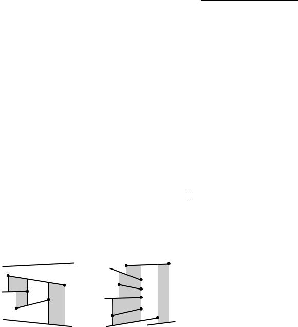
So we have a set S of n non-crossing line segments, enclosed in a bounding box R, and with the property that no two distinct endpoints lie on a common vertical line. We call such a set a set of line segments in general position. The trapezoidal map T(S) of S—also known as the vertical decomposition or trapezoidal decomposition of S—is obtained by drawing two vertical extensions from every endpoint p of a segment in S, one extension going upwards and one going downwards. The extensions stop when they meet another segment of S or the boundary of R. We call the two vertical extensions starting in an endpoint p the upper vertical extension and the lower vertical extension. The trapezoidal map of S is simply the subdivision induced by S, the rectangle R, and the upper and lower vertical extensions. Figure 6.3 shows an example.
R
A face in T(S) is bounded by a number of edges of T(S). Some of these edges may be adjacent and collinear. We call the union of such edges a side of the face. In other words, the sides of a face are the segments of maximal length that are contained in the boundary of a face.
Lemma 6.1 Each face in a trapezoidal map of a set S of line segments in general position has one or two vertical sides and exactly two non-vertical sides.
Proof. Let f be a face in T(S). We first prove that f is convex.
Because the segments in S are non-crossing, any corner of f is either an endpoint of a segment in S, a point where a vertical extension abuts a segment of S or an edge of R, or it is a corner of R. Due to the vertical extensions, no corner that is a segment endpoint can have an interior angle greater than 180◦. Moreover, any angle at a point where a vertical extension abuts a segment must be less than or equal to 180◦ as well. Finally, the corners of R are 90◦. Hence, f is convex—the vertical extensions have removed all non-convexities.
Because we are looking at sides of f , rather than at edges of T(S) on the boundary of f , the convexity of f implies that it can have at most two vertical sides. Now suppose for a contradiction that f has more than two non-vertical sides. Then there must be two such sides that are adjacent and either both bound f from above or both bound f from below. Because any non-vertical side must be contained in a segment of S or in an edge of R, and the segments are non-crossing, the two adjacent sides must meet in a segment endpoint. But then the vertical extensions for that endpoint prevent the two sides from being adjacent, a contradiction. Hence, f has at most two non-vertical sides.
Finally, we observe that f is bounded (since we have enclosed the whole scene in a bounding box R), which implies that it cannot have less than two non-vertical sides and that it must have at least one vertical side. 

Section 6.1
POINT LOCATION AND TRAPEZOIDAL
MAPS
Figure 6.3
A trapezoidal map
 sides
sides
125
Chapter 6
POINT LOCATION
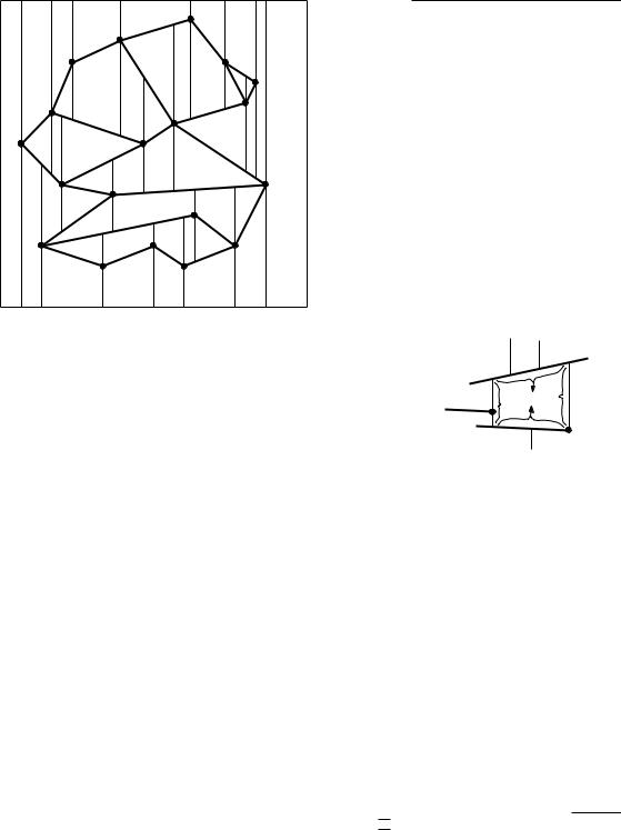
top(∆)
∆
bottom(∆)
Figure 6.4
Four of the five cases for the left edge of trapezoid ∆
Lemma 6.1 shows that the trapezoidal map deserves its name: each face is either a trapezoid or a triangle, which we can view as a trapezoid with one degenerate edge of length zero.
In the proof of Lemma 6.1 we observed that a non-vertical side of a trapezoid is contained in a segment of S or in a horizontal edge of R. We denote the nonvertical segment of S, or edge of R, bounding a trapezoid ∆ from above by top(∆), and the one bounding it from below by bottom(∆).
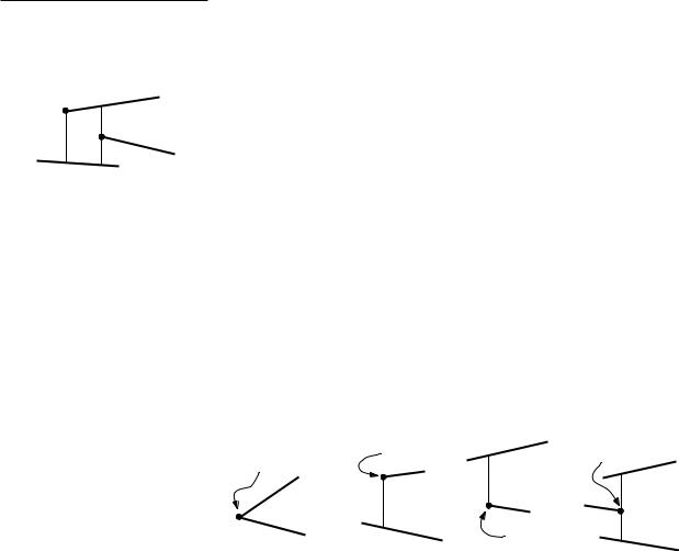
By the general position assumption, a vertical side of a trapezoid either consists of vertical extensions, or it is the vertical edge of R. More precisely, we can distinguish five different cases for the left side and the right side of a trapezoid ∆. The cases for the left side are as follows:
(a)It degenerates to a point, which is the common left endpoint of top(∆) and bottom(∆).
(b)It is the lower vertical extension of the left endpoint of top(∆) that abuts on bottom(∆).
(c)It is the upper vertical extension of the left endpoint of bottom(∆) that abuts on top(∆).
(d)It consists of the upper and lower extension of the right endpoint p of a third segment s. These extensions abut on top(∆) and bottom(∆), respectively.
(e)It is the left edge of R. This case occurs for a single trapezoid of T(S) only, namely the unique leftmost trapezoid of T(S).
The first four cases are illustrated in Figure 6.4. The five cases for the right vertical edge of ∆ are symmetrical. You should verify for yourself that the listing above is indeed exhaustive.
leftp(∆) |
leftp(∆) |
top(∆) |
leftp(∆) |
|
|
||
|
top(∆) |
|
top(∆) |
top(∆) |
|
|
|
|
bottom(∆) |
s |
|
bottom(∆) |
bottom(∆) |
|
|
|
|
bottom(∆) |
|
|
|
leftp(∆) |
|
(a) |
(b) |
(c) |
(d) |
For every trapezoid ∆ T(S), except the leftmost one, the left vertical edge of ∆ is, in a sense, defined by a segment endpoint p: it is either contained in the vertical extensions of p, or—when it is degenerate—it is p itself. We will
|
denote the endpoint defining the left edge of ∆ by leftp(∆). As shown above, |
|
leftp(∆) is the left endpoint of top(∆) or bottom(∆), or it is the right endpoint |
|
of a third segment. For the unique trapezoid whose left side is the left edge of |
|
R, we define leftp(∆) to be the lower left vertex of R. Similarly, we denote the |
|
endpoint that defines the right vertical edge of ∆ by rightp(∆). Notice that ∆ is |
|
uniquely determined by top(∆), bottom(∆), leftp(∆), and rightp(∆). Therefore |
|
we will sometimes say that ∆ is defined by these segments and endpoints. |
|
The trapezoidal map of the edges of a subdivision is a refinement of that |
126 |
subdivision. It is not clear, however, why point location in a trapezoidal map |
should be any easier than point location in a general subdivision. But before we come to this in the next section, let’s first verify that the complexity of the trapezoidal map is not too much larger than the number of segments in the set defining it.
Lemma 6.2 The trapezoidal map T(S) of a set S of n line segments in general position contains at most 6n + 4 vertices and at most 3n + 1 trapezoids.
Proof. A vertex of T(S) is either a vertex of R, an endpoint of a segment in S, or else the point where the vertical extension starting in an endpoint abuts on another segment or on the boundary of R. Since every endpoint of a segment induces two vertical extensions—one upwards, one downwards—this implies that the total number of vertices is bounded by 4 + 2n + 2(2n) = 6n + 4.
A bound on the number of trapezoids follows from Euler’s formula and the bound on the number of vertices. Here we give a direct proof, using the point leftp(∆). Recall that each trapezoid has such a point leftp(∆). This point is the endpoint of one of the n segments, or is the lower left corner of R. By looking at the five cases for the left side of a trapezoid, we find that the lower left corner of R plays this role for exactly one trapezoid, a right endpoint of a segment can play this role for at most one trapezoid, and a left endpoint of a segment can be the leftp(∆) of at most two different trapezoids. (Since endpoints can coincide, a point in the plane can be leftp(∆) for many trapezoids. However, if in case (a) we consider leftp(∆) to be the left endpoint of bottom(∆), then the left endpoint of a segment s can be leftp(∆) for only two trapezoids, one above s and one below s.) It follows that the total number of trapezoids is at most 3n + 1. 

We call two trapezoids ∆ and ∆ adjacent if they meet along a vertical edge. In Figure 6.5(i), for example, trapezoid ∆ is adjacent to ∆1, ∆2, and ∆3, but not to ∆4 and ∆5. Because the set of line segments is in general position, a trapezoid has at most four adjacent trapezoids. If the set is not in general position, a trapezoid can have an arbitrary number of adjacent trapezoids, as illustrated in Figure 6.5(ii). Let ∆ be a trapezoid that is adjacent to ∆ along the left vertical
Section 6.1
POINT LOCATION AND TRAPEZOIDAL
MAPS
(i) |
|
|
(ii) |
|
∆1 |
|
|
|
|
|
|||
|
|
|
|
|
|
|
|
||||||
|
|
|
∆5 |
|
|
|
|
|
|
|
|
||
|
|
|
|
|
|
|
|||||||
|
|
|
|
|
|
|
|
|
|
|
|||
|
|
∆1 |
|
|
|
∆2 |
|
|
|
|
|
||
|
|
|
|
|
|
|
|
|
|
||||
|
|
|
|
|
|
|
|
|
|
||||
|
|
|
|
|
∆3 |
|
|
|
|
|
|||
|
|
∆2 |
∆ |
∆3 |
|
∆ |
∆6 |
|
|
|
|||
|
|
|
|
|
|||||||||
|
|
|
|
∆4 |
|
|
|
|
|
||||
|
|
|
|
|
|
|
|
|
|
||||
|
|
|
∆4 |
|
|
|
|
|
|
|
|||
|
|
|
|
|
∆5 |
|
|
|
Figure 6.5 |
||||
|
|
|
|
|
|
|
|
|
|||||
|
|
|
|
|
|
|
|
|
|
|
Trapezoids adjacent to ∆ are shaded |
||
edge of ∆. Then either top(∆) = top(∆ ) or bottom(∆) = bottom(∆ ). In the first |
|||||||||||||
|
|
||||||||||||
case we call ∆ the upper left neighbor of ∆, and in the second case ∆ is the |
|
|
|||||||||||
lower left neighbor of ∆. So the trapezoid in Figure 6.4(b) has a bottom left |
|
|
|||||||||||
neighbor but no top left neighbor, the trapezoid in Figure 6.4(c) has a top left |
|
|
|||||||||||
neighbor but no bottom left neighbor, and the trapezoid in Figure 6.4(d) has both |
|
|
|||||||||||
a top left neighbor and a bottom left neighbor. The trapezoid in Figure 6.4(a) |
127 |
||||||||||||

Chapter 6
POINT LOCATION
and the single trapezoid whose left vertical edge is the left side of R have no left neighbors. The upper right neighbor and lower right neighbor of a trapezoid are defined similarly.
To represent a trapezoidal map, we could use the doubly-connected edge list described in Chapter 2; after all, a trapezoidal map is a planar subdivision. However, the special shape of the trapezoidal map makes it more convenient to use a specialized structure. This structure uses the adjacency of trapezoids to link the subdivision as a whole. There are records for all line segments and endpoints of S, since they serve as leftp(∆), rightp(∆), top(∆), and bottom(∆). Furthermore, the structure contains records for the trapezoids of T(S), but not for edges or vertices of T(S). The record for a trapezoid ∆ stores pointers to top(∆) and bottom(∆), pointers to leftp(∆) and rightp(∆), and finally, pointers to its at most four neighbors. Note that the geometry of a trapezoid ∆ (that is, the coordinates of its vertices) is not available explicitly. However, ∆ is uniquely defined by top(∆), bottom(∆), leftp(∆), and rightp(∆). This means that we can deduce the geometry of ∆ in constant time from the information stored for ∆.
6.2 A Randomized Incremental Algorithm
In this section we will develop a randomized incremental algorithm that constructs the trapezoidal map T(S) of a set S of n line segments in general position. During the construction of the trapezoidal map, the algorithm also builds a data structure D that can be used to perform point location queries in T(S). This is the reason why a plane sweep algorithm isn’t chosen to construct the trapezoidal map. It would construct it all right, but it wouldn’t give us a data structure that supports point location queries, which is the main objective of this chapter.
|
Before discussing the algorithm, we first describe the point location data struc- |
|
ture D that the algorithm constructs. This structure, which we call the search |
|
structure, is a directed acyclic graph with a single root and exactly one leaf for |
|
every trapezoid of the trapezoidal map of S. Its inner nodes have out-degree 2. |
|
There are two types of inner nodes: x-nodes, which are labeled with an endpoint |
|
of some segment in S, and y-nodes, which are labeled with a segment itself. |
|
A query with a point q starts at the root and proceeds along a directed path |
|
to one of the leaves. This leaf corresponds to the trapezoid ∆ T(S) containing |
|
q. At each node on the path, q has to be tested to determine in which of the two |
|
child nodes to proceed. At an x-node, the test is of the form: “Does q lie to the |
|
left or to the right of the vertical line through the endpoint stored at this node?” |
|
At a y-node, the test has the form: “Does q lie above or below the segment s |
|
stored here?” We will ensure that whenever we come to a y-node, the vertical |
|
line through q intersects the segment of that node, so that the test makes sense. |
|
The tests at the inner nodes only have two outcomes: left or right of an endpoint |
|
for an x-node, and above or below a segment for a y-node. What should we |
|
do if the query point lies exactly on the vertical line, or on the segment? For |
128 |
now, we shall simply make the assumption that this does not occur; Section 6.3, |
which shows how to deal with sets of segments that are not in general position, will also deal with this type of query point.
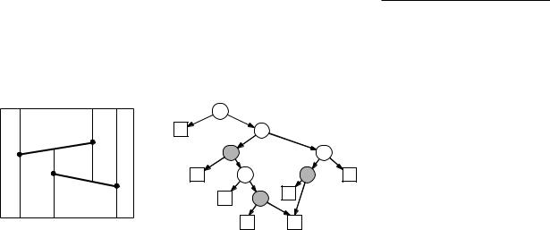
The search structure D and the trapezoidal map T(S) computed by the algorithm are interlinked: a trapezoid ∆ T(S) has a pointer to the leaf of D corresponding to it, and a leaf node of D has a pointer to the corresponding trapezoid in T(S). Figure 6.6 shows the trapezoidal map of a set of two line
Section 6.2
A RANDOMIZED INCREMENTAL
ALGORITHM
p1 |
B |
s1 |
q1 |
A |
q1 |
p1 |
s1 |
|
||
D |
E |
|
||
|
G |
|
||
p2 |
s2 |
|
B |
p2 |
A |
|
|
q2 |
|
C |
|
|
s2 |
|
F |
|
C |
||
|
|
|
|
D |
q2 |
s2 |
G |
E
F
Figure 6.6
The trapezoidal map of two segments and a search structure
segments s1 and s2, and a search structure for the trapezoidal map. The x-nodes are white, with the endpoint labeling it inside. The y-nodes are grey and have the segment labeling it inside. The leaves of the search structure are shown as squares, and are labeled with the corresponding trapezoid in the trapezoidal map.
The algorithm we give for the construction of the search structure is incremental: it adds the segments one at a time, and after each addition it updates the search structure and the trapezoidal map. The order in which the segments are added influences the search structure; some orders lead to a search structure with a good query time, while for others the query time will be bad. Instead of trying to be clever in finding a suitable order, we shall take the same approach we took in Chapter 4, where we studied linear programming: we use a random ordering. So the algorithm will be randomized incremental. Later we will prove that the search structure resulting from a randomized incremental algorithm is expected to be good. But first we describe the algorithm in more detail. We begin with its global structure; the various substeps will be explained after that.
Algorithm TRAPEZOIDALMAP(S)
Input. A set S of n non-crossing line segments.
Output. The trapezoidal map T(S) and a search structure D for T(S) in a bounding box.
1.Determine a bounding box R that contains all segments of S, and initialize the trapezoidal map structure T and search structure D for it.
2.Compute a random permutation s1, s2, . . . , sn of the elements of S.
3.for i ← 1 to n
4.do Find the set ∆0, ∆1, . . . , ∆k of trapezoids in T properly intersected
|
by si. |
|
|
5. |
Remove ∆0, ∆1, . . . , ∆k from T and replace them by the new trape- |
|
|
|
|
||
|
zoids that appear because of the insertion of si. |
129 |
|

Chapter 6
POINT LOCATION
∆0 ∆1 |
∆3 |
si ∆2
130
6.Remove the leaves for ∆0, ∆1, . . . , ∆k from D, and create leaves for the new trapezoids. Link the new leaves to the existing inner nodes by adding some new inner nodes, as explained below.
We now describe the various steps of the algorithm in more detail. In the following, we let Si := {s1, s2, . . . , si}. The loop invariant of TRAPEZOIDALMAP is that T is the trapezoidal map for Si, and that D is a valid search structure for T.
The initialization of T as T(S0) = T(0/) and of D in line 1 is easy: the trapezoidal map for the empty set consists of a single trapezoid—the bounding rectangle R—and the search structure for T(0/) consists of a single leaf node for this trapezoid. For the computation of the random permutation in line 2 see Chapter 4. Now let’s see how to insert a segment si in lines 4–6.
To modify the current trapezoidal map, we first have to know where it changes. This is exactly at the trapezoids that are intersected by si. Stated more precisely, a trapezoid of T(Si−1) is not present in T(Si) if and only if it is intersected by si. Our first task is therefore to find the intersected trapezoids. Let ∆0, ∆1, . . . , ∆k denote these trapezoids, ordered from left to right along si. Observe that ∆j+1 must be one of the right neighbors of ∆j. It is also easy to test which neighbor it is: if rightp(∆j) lies above si, then ∆j+1 is the lower right neighbor of ∆j, otherwise it is the upper right neighbor. This means that once we know ∆0, we can find ∆1, . . . , ∆k by traversing the representation of the trapezoidal map. So, to get started, we need to find the trapezoid ∆0 T containing the left endpoint, p, of si. If p is not yet present in Si−1 as an endpoint, then, because of our general position assumption, it must lie in the interior of ∆0. This means we can find ∆0 by a point location with p in T(Si−1). And now comes the exciting part: at this stage in the algorithm D is a search structure for T = T(Si−1), so all that we need to do is to perform a query on D with the point p.
If p is already an endpoint of a segment in Si−1—remember that we allow different segments to share an endpoint—then we must be careful. To find ∆0, we simply start to search in D. If p happens not to be present yet, then the query algorithm will proceed without trouble, and end up in the leaf corresponding to ∆0. If, however, p is already present, then the following will happen: at some point during the search, p will lie on the vertical line through the point in an x-node. Recall that we decided that such query points are illegal. To remedy this, we should imagine continuing the query with a point p slightly to the right of p. Replacing p by p is only done conceptually. What it actually means when implementing the search is this: whenever p lies on the vertical line of an x-node, we decide that it lies to the right. Similarly, whenever p lies on a segment s of a y-node (this can only happen if si shares its left endpoint, p, with s) we compare the slopes of s and si; if the slope of si is larger, we decide that p lies above s, otherwise we decide that it is below s. With this adaptation, the search will end in the first trapezoid ∆0 intersected properly by si. In summary, we use the following algorithm to find ∆0, . . . , ∆k.
Algorithm FOLLOWSEGMENT(T, D, si)
Input. A trapezoidal map T, a search structure D for T, and a new segment si. Output. The sequence ∆0, . . . , ∆k of trapezoids intersected by si.
1.Let p and q be the left and right endpoint of si.
2.Search with p in the search structure D to find ∆0.
3.j ← 0;
4.while q lies to the right of rightp(∆j)
5.do if rightp(∆j) lies above si
6.then Let ∆j+1 be the lower right neighbor of ∆j.
7.else Let ∆j+1 be the upper right neighbor of ∆j.
8.j ← j + 1
9.return ∆0, ∆1, . . . , ∆j
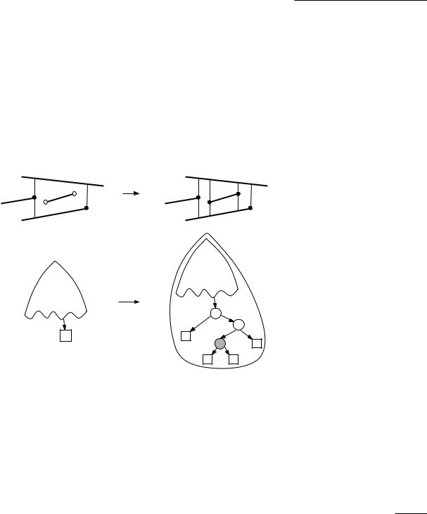
We have seen how to find the trapezoids intersecting si. The next step is to update T and D. Let’s start with the simple case that si is completely contained in a trapezoid ∆ = ∆0. We are in the situation depicted on the left hand side of Figure 6.7.
Section 6.2
A RANDOMIZED INCREMENTAL
ALGORITHM
T(Si−1) |
|
T(Si) |
|
∆ |
A |
C |
|
si qi |
B |
||
|
|||
pi |
|
D |
D(Si−1) D(Si)
D(Si−1)
|
pi |
|
|
|
qi |
∆ |
A |
B |
|
si |
|
|
C |
D |
To update T, we delete ∆ from T, and replace it by four new trapezoids A, B, C, and D. Notice that all the information we need to initialize the records for the new trapezoids correctly (their neighbors, the segments on the top and bottom, and the points defining their left and right vertical edges) are available: they can be determined in constant time from the segment si and the information stored for ∆.
It remains to update D. What we must do is replace the leaf for ∆ by a little tree with four leaves. The tree contains two x-nodes, testing with the left and right endpoint of si, and one y-node, testing with the segment si itself. This is sufficient to determine in which of the four new trapezoids A, B, C, or D a query point lies, if we already know that it lies in ∆. The right hand side of Figure 6.7 illustrates the modifications to the search structure. Note that one or both endpoints of the segment si could be equal to leftp(∆) or rightp(∆). In that
Figure 6.7
The new segment si lies completely in trapezoid ∆
131
Chapter 6
POINT LOCATION
case there would be only two or three new trapezoids, but the modification is done in the same spirit.
The case where si intersects two or more trapezoids is only slightly more complicated. Let ∆0, ∆1, . . . , ∆k be the sequence of intersected trapezoids. To update T, we first erect vertical extensions through the endpoints of si,
|
|
T(S |
i−1 |
) |
|
|
T(Si) |
∆0 |
|
|
|
|
|
|
|
∆2 |
qi |
|
|
|
D |
E |
|
|
|
|
|
||||
pi |
∆1 |
∆3 |
|
|
A |
F |
|
|
|
B |
C |
||||
|
|
|
|
|
|||
si |
si |
Figure 6.8
Segment si intersects four trapezoids
132
D(Si)
D(Si−1) |
D(Si−1) |
∆0 ∆1 |
∆2 |
si |
si |
si |
|
qi |
∆3 |
|
|
|
|
||
|
|
B |
|
D |
si |
F |
|
|
|
|
E
A
C
partitioning ∆0 and ∆k into three new trapezoids each. This is only necessary for the endpoints of si that were not already present. Then we shorten the vertical extensions that now abut on si. This amounts to merging trapezoids along the segment si, see Figure 6.8. Using the information stored with the trapezoids ∆0, ∆1, . . . , ∆k, this step can be done in time that is linear in the number of intersected trapezoids.
To update D, we have to remove the leaves for ∆0, ∆1, . . . , ∆k, we must create leaves for the new trapezoids, and we must introduce extra inner nodes. More precisely, we proceed as follows. If ∆0 has the left endpoint of si in its interior (which means it has been partitioned into three new trapezoids) then we replace the leaf for ∆0 with an x-node for the left endpoint of si and a y-node for the segment si. Similarly, if ∆k has the right endpoint of si in its interior, we replace the leaf for ∆k with an x-node for the right endpoint of si and a y-node for si. Finally, the leaves of ∆1 to ∆k−1 are replaced with single y-nodes for the segment si. We make the outgoing edges of the new inner nodes point to the

correct new leaves. Notice that, due to the fact that we have merged trapezoids stemming from different trapezoids of T, there can be several incoming edges for a new trapezoid. Figure 6.8 illustrates this.
We have finished the description of the algorithm that constructs T(s) and, at the same time, builds a search structure D for it. The correctness of the algorithm follows directly from the loop invariant (stated just after Algorithm TRAPEZOIDALMAP), so it remains to analyze its performance.
The order in which we treat the segments has considerable influence on the resulting search structure D and on the running time of the algorithm itself. For some cases the resulting search structure has quadratic size and linear search time, but for other permutations of the same set of segments the resulting search structure is much better. As in Chapter 4, we haven’t tried to determine a good sequence; we simply took a random insertion sequence. This means that the analysis will be probabilistic: we shall look at the expected performance of the algorithm and of the search structure. Perhaps it’s not quite clear yet what the term “expected” means in this context. Consider a fixed set S of n non-crossing line segments. TRAPEZOIDALMAP computes a search structure D for T(S). This structure depends on the permutation chosen in line 2. Since there are n! possible permutations of n objects, there are n! possible ways in which the algorithm can proceed. The expected running time of the algorithm is the average of the running time, taken over all n! permutations. For each permutation, a different search structure will result. The expected size of D is the average of the sizes of all these n! search structures. Finally, the expected query time for a point q is the average of the query time for point q, over all n! search structures. (Notice that this not the same as the average of the maximum query time for the search structure. Proving a bound on this quantity is a bit more technical, so we defer that to Section 6.4.)
Theorem 6.3 Algorithm TRAPEZOIDALMAP computes the trapezoidal map T(S) of a set S of n line segments in general position and a search structure D for T(S) in O(n log n) expected time. The expected size of the search structure is O(n) and for any query point q the expected query time is O(log n).
Proof. As noted earlier, the correctness of the algorithm follows directly from the loop invariant, so we concentrate on the performance analysis.
We start with the query time of the search structure D. Let q be a fixed query point. As the query time for q is linear in the length of the path in D that is traversed when querying with q, it suffices to bound the path length. A simple case analysis shows that the depth of D (that is, the maximum path length) increases by at most 3 in every iteration of the algorithm. Hence, 3n is an upper bound on the query time for q. This bound is the best possible worst-case bound over all possible insertion orders for S. We are not so much interested in the worst-case case behavior, however, but in the expected behavior: we want to bound the average query time for q with respect to the n! possible insertion orders.
Consider the path traversed by the query for q in D. Every node on this path was created at some iteration of the algorithm. Let Xi, for 1 i n, denote
Section 6.2
A RANDOMIZED INCREMENTAL
ALGORITHM
133
Chapter 6
POINT LOCATION
134
the number of nodes on the path created in iteration i. Since we consider S and q to be fixed, Xi is a random variable—it depends on the random order of the segments only. We can now express the expected path length as
n |
n |
E[∑Xi] = ∑E[Xi]. |
|
i=1 |
i=1 |
The equality here is linearity of expectation: the expected value of a sum is equal to the sum of the expected values.
We already observed that any iteration adds at most three nodes to the search path for any possible query point, so Xi 3. In other words, if Pi denotes the probability that there exists a node on the search path of q that is created in iteration i, we have
E[Xi] 3Pi.
The central observation to derive a bound on Pi is this: iteration i contributes a node to the search path of q exactly if ∆q(Si−1), the trapezoid containing q in T(Si−1), is not the same as ∆q(Si), the trapezoid containing q in T(Si). In other
words,
Pi = Pr[∆q(Si) =∆q(Si−1)].
If ∆q(Si) is not the same as ∆q(Si−1), then ∆q(Si) must be one of the trapezoids created in iteration i. Note that all trapezoids ∆ created in iteration i are adjacent to si, the segment that is inserted in that iteration: either top(∆) or bottom(∆) is si, or leftp(∆) or rightp(∆) is an endpoint of si.
Now consider a fixed set Si S. The trapezoidal map T(Si), and therefore ∆q(Si), are uniquely defined as a function of Si; ∆q(Si) does not depend on the order in which the segments in Si have been inserted. To bound the probability that the trapezoid containing q has changed due to the insertion of si, we shall use a trick we also used in Chapter 4, called backwards analysis: we consider T(Si) and look at the probability that ∆q(Si) disappears from the trapezoidal map
when we remove the segment si. By what we said above, ∆q(Si) disappears if and only if one of top(∆q(Si)), bottom(∆q(Si)), leftp(∆q(Si)), or rightp(∆q(Si))
disappears with the removal of si. What is the probability that top(∆q(Si)) disappears? The segments of Si have been inserted in random order, so every segment in Si is equally likely to be si. This means that the probability that si happens to be top(∆q(Si)) is 1/i. (If top(∆q(Si)) is the top edge of the rectangle R surrounding the scene, then the probability is even zero.) Similarly, the probability that si happens to be bottom(∆q(Si)) is at most 1/i. There can be many segments sharing the point leftp(∆q(Si)). Hence, the probability that si is one of these segments can be large. But leftp(∆q(Si)) disappears only if si is the only segment in Si with leftp(∆q(Si)) as an endpoint. Hence, the probability that leftp(∆q(Si)) disappears is at most 1/i as well. The same holds true for rightp(∆q(Si)). Hence, we can conclude that
Pi = Pr[∆q(Si) =∆q(Si−1)] = Pr[∆q(Si) T(Si−1)] 4/i.
(A small technical point: In the argument above we fixed the set Si. This means that the bound we derived on Pi holds under the condition that Si is this fixed

set. But since the bound does not depend on what the fixed set actually is, the bound holds unconditionally.)
Putting it all together we get the bound on the expected query time:
n |
n |
n |
12 |
n |
1 |
|
|||
E[∑Xi] ∑ |
3Pi ∑ |
= 12 ∑ |
= 12Hn. |
||||||
|
i |
|
i |
||||||
i=1 |
i=1 |
i=1 |
|
i=1 |
|
|
|||
|
|
|
|
|
|||||
Here, Hn is the n-th harmonic number, defined as
|
1 |
|
1 |
|
1 |
1 |
||||
Hn := |
|
+ |
|
|
+ |
|
|
+ ···+ |
|
|
1 |
|
2 |
|
3 |
n |
|||||
Harmonic numbers arise quite often in the analysis of algorithms, so it’s good to remember the following bound that holds for all n > 1:
ln n < Hn < ln n + 1.
(It can be derived by comparing Hn to the integral n 1/x dx = ln n.) We
1
conclude that the expected query time for a query point q is O(log n), as claimed. Let’s now turn to the size of D. To bound the size, it suffices to bound the number of nodes in D. We first note that the leaves in D are in one-to-one correspondence with the trapezoids in ∆, of which there are O(n) by Lemma 6.2.
This means that the total number of nodes is bounded by
n
O(n) + ∑(number of inner nodes created in iteration i).
i=1
Let ki be the number of new trapezoids that are created in iteration i, due to the insertion of segment si. In other words, ki is the number of new leaves in D. The number of inner nodes created in iteration i is exactly equal to ki − 1. A simple worst case upper bound on ki follows from the fact that the number of new trapezoids in T(Si) can obviously not be larger than the total number of trapezoids in T(Si), which is O(i). This leads to a worst-case upper bound on the size of the structure of
n
O(n) + ∑O(i) = O(n2).
i=1
Indeed, if we have bad luck and the order in which we insert the segments is very unfortunate, then the size of D can be quadratic. However, we are more interested in the expected size of the data structure, over all possible insertion orders. Using linearity of expectation, we find that this expected size is bounded by
n |
n |
O(n) + E[∑(ki −1)] = O(n) + ∑E[ki]. |
|
i=1 |
i=1 |
It remains to bound the expected value of ki. We already prepared the necessary tools for this when we derived the bound on the query time. Consider a fixed
set Si S. For a trapezoid ∆ T(Si) and a segment s Si, let
1 if ∆ disappears from T(Si) when s is removed from Si,
0 otherwise.
Section 6.2
A RANDOMIZED INCREMENTAL
ALGORITHM
135

Chapter 6
POINT LOCATION
In the analysis of the query time we observed that there are at most four segments that cause a given trapezoid to disappear. Hence,
∑ ∑ δ (∆, s) 4|T(Si)| = O(i).
s Si ∆ T(Si)
Now, ki is the number of trapezoids created by the insertion of si, or, equivalently, the number of trapezoids in T(Si) that disappear when si is removed. Since si is a random element of Si, we can find the expected value of ki by taking the average over all s Si:
E[ki] = |
1 |
∑ ∑ |
δ (∆, s) |
O(i) |
|
= O(1). |
|
|
i |
i |
|
||||
|
|
s Si ∆ T(Si) |
|
|
|||
|
|
|
|
|
|
|
|
We conclude that the expected number of newly created trapezoids is O(1) in every iteration of the algorithm, from which the O(n) bound on the expected amount of storage follows.
It remains to bound the expected running time of the construction algorithm. Given the analysis of the query time and storage, this is easy. We only need to observe that the time to insert segment si is O(ki) plus the time needed to locate the left endpoint of si in T(Si−1). Using the earlier derived bounds on ki and the query time, we immediately get that the expected running time of the algorithm is
= O(n log n).
This completes the proof.
Note once again that the expectancy in Theorem 6.3 is solely with respect to the random choices made by the algorithm; we do not average over possible choices for the input. Hence, there are no bad inputs: for any input set of n line segments, the expected running time of the algorithm is O(n log n).
As discussed earlier, Theorem 6.3 does not guarantee anything about the expected maximum query time over all possible query points. In Section 6.4, however, it is proved that the expected maximum query time is O(log n) as well. Hence, we can build a data structure of expected size O(n), whose expected query time is O(log n). This also proves the existence of a data structure with O(n) size and O(log n) query time for any query point q—see Theorem 6.8.
|
Finally we go back to our original problem: point location in a planar subdivi- |
|
sion S. We assume that S is given as a doubly-connected edge list with n edges. |
|
We use algorithm TRAPEZOIDALMAP to compute a search structure D for the |
|
trapezoidal map of the edges of S. To use this search structure for point location |
|
in S, however, we still need to attach to every leaf of D a pointer to the face f |
|
of S that contains the trapezoid of T(S) corresponding to that leaf. But this |
|
is rather easy: recall from Chapter 2 that the doubly-connected edge list of S |
136 |
stores with every half-edge a pointer to the face that is incident to the left. The |
face that is incident to the right can be found in constant time from Twin(e). So for every trapezoid ∆ of T(S) we simply look at the face of S incident to top(∆) from below. If top(∆) is the top edge of R, then ∆ is contained in the unique unbounded face of S.
In the next section we show that the assumption that the segments be in general position may be dropped, which leads to a less restricted version of Theorem 6.3. It implies the following corollary.
Corollary 6.4 Let S be a planar subdivision with n edges. In O(n log n) expected time one can construct a data structure that uses O(n) expected storage, such that for any query point q, the expected time for a point location query is O(log n).
Section 6.3
DEALING WITH DEGENERATE CASES
6.3Dealing with Degenerate Cases
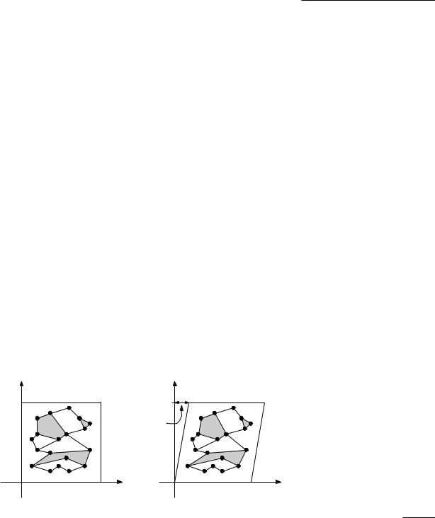
In the previous sections we made two simplifying assumptions. First of all, we assumed that the set of line segments was in general position, meaning that no two distinct endpoints have the same x-coordinate. Secondly, we assumed that a query point never lies on the vertical line of an x-node on its search path, nor on the segment of a y-node. We now set out to get rid of these assumptions.
We first show how to avoid the assumption that no two distinct endpoints lie on a common vertical line. The crucial observation is that the vertical direction chosen to define the trapezoidal map of the set of line segments was immaterial. Therefore we can rotate the axis-system slightly. If the rotation angle is small enough, then no two distinct endpoints will lie on the same vertical line anymore. Rotations by very small angles, however, lead to numerical difficulties. Even if the input coordinates are integer, we need a significantly higher precision to do the calculations properly. A better approach is to do the rotation symbolically. In Chapter 5 we have seen another form of a symbolic transformation, composite numbers, which was used to deal with the case where data points have the same x- or y-coordinate. In this chapter, we will have another look at such a symbolic perturbation, and will try to interpret it geometrically.
y |
y |
|
1 |
|
ε |
|
ϕ |
|
→ |
x |
x |
Figure 6.9
The shear transformation
It will be convenient not to use rotation, but to use an affine mapping called |
|
shear transformation. In particular, we shall use the shear transformation along |
137 |

Chapter 6
POINT LOCATION
138
the x-axis by some value ε > 0: |
|
|
|
|
|
|
x + ε y |
||
ϕ : |
x |
→ |
. |
|
y |
y |
|||
Figure 6.9 illustrates the effect of this shear transform. It maps a vertical line to a line with slope 1/ε , so that any two distinct points on the same vertical line are mapped to points with distinct x-coordinates. Furthermore, if ε > 0 is small enough, then the transformation does not reverse the order in x-direction of the given input points. It is not difficult to compute an upper bound for ε to guarantee that this property holds. In the following, we will assume that we have a value of ε > 0 available that is small enough that the order of points is conserved by the shear transform. Surprisingly, we will later realize that we do not need to compute such an actual value for ε .
Given a set S of n arbitrary non-crossing line segments, we will run algorithm TRAPEZOIDALMAP on the set ϕ S := {ϕ s : s S}. As noted earlier, however, actually performing the transformation may lead to numerical problems, and therefore we use a trick: a point ϕ p = (x + ε y, y) will simply be stored as (x, y). This is a unique representation. We only need to make sure that the algorithm treats the segments represented in this way correctly. Here it comes handy that the algorithm does not compute any geometric objects: we never actually compute the coordinates of the endpoints of vertical extensions, for instance. All it does is to apply two types of elementary operations to the input points. The first operation takes two distinct points p and q and decides whether q lies to the left, to the right, or on the vertical line through p. The second operation takes one of the input segments, specified by its two endpoints p1 and p2, and tests whether a third point q lies above, below, or on this segment. This second operation is only applied when we already know that a vertical line through q intersects the segment. All the points p, q, p1, and p2 are endpoints of segments in the input set S. (You may want to go through the description of the algorithm again, verifying that it can indeed be realized with these two operations alone.)
Let’s look at how to apply the first operation to two transformed points ϕ p and ϕ q. These points have coordinates (xp + ε yp, yp) and (xq + ε yq, yq), respectively. If xq =xp, then the relation between xq and xp determines the outcome of the test—after all, we had chosen ε to have this property. If xq = xp, then the relation between yq and yp decides the horizontal order of the points. Therefore there is a strict horizontal order for any pair of distinct points. It follows that ϕ q will never lie on the vertical line through ϕ p, except when p and q coincide. But this is exactly what we need, since no two distinct input points should have the same x-coordinate.
For the second operation, we are given a segment ϕ s with endpoints ϕ p1 = (x1 + ε y1, y1) and ϕ p2 = (x2 + ε y2, y2), and we want to test whether a point ϕ q = (x + ε y, y) lies above, below, or on ϕ s. The algorithm ensures that whenever we do this test, the vertical line through ϕ q intersects ϕ s. In other words,
x1 + ε y1 x + ε y x2 + ε y2.

This implies that x1 x x2. Moreover, if x = x1 then y y1, and if x = x2 then y y2. Let’s now distinguish two cases.
If x1 = x2, the untransformed segment s is vertical. Since now x1 = x = x2, we have y1 y y2, which implies that q lies on s. Because the affine mapping ϕ is incidence preserving—if two points coincide before the transformation, they do so afterwards—we can conclude that ϕ q lies on ϕ s.
Now consider the case where x1 < x2. Since we already know that the vertical line through ϕ q intersects ϕ s, it is good enough to do the test with ϕ s. Now we observe that the mapping ϕ preserves the relation between points and lines: if a point is above (or on, or below) a given line, then the transformed point is above (or on, or below) the transformed line. Hence, we can simply perform the test with the untransformed point q and segment s.
This shows that to run the algorithm on ϕ S instead of on S, the only modification we have to make is to compare points lexicographically, when we want to determine their horizontal order. Of course, the algorithm will compute the trapezoidal map for ϕ S, and a search structure for T(ϕ S). Note that, as promised, we never actually needed the value of ε , so there is no need to compute such a value at the beginning. All we needed was that ε is small enough.
Using our shear transformation, we got rid of the assumption that any two distinct endpoints should have distinct x-coordinates. What about the restriction that a query point never lies on the vertical line of an x-node on the search path, nor on the segment of a y-node? Our approach solves this problem as well, as we show next.
Since the constructed search structure is for the transformed map T(ϕ S), we will also have to use the transformed query point ϕ q when doing a query. In other words, all the comparisons we have to do during the search must be done in the transformed space. We already know how to do the tests in the transformed space:
At x-nodes we have to do the test lexicographically. As a result, no two distinct points will ever lie on a vertical line. (Trick question: How can this be true, if the transformation ϕ is bijective?) This does not mean that the outcome of the test at an x-node is always “to the right” or “to the left”. The outcome can also be “on the line”. This can only happen, however, when the query point coincides with the endpoint stored at the node—and this answers the query!
At y-nodes we have to test the transformed query point against a transformed segment. The test described above can have three outcomes: “above”, “below”, or “on”. In the first two cases, there is no problem, and we can descend to the corresponding child of the y-node. If the outcome of the test is “on”, then the untransformed point lies on the untransformed segment as well, and we can report that fact as the answer to the query.
We have generalized Theorem 6.3 to arbitrary sets of non-crossing line segments.
Theorem 6.5 Algorithm TRAPEZOIDALMAP computes the trapezoidal map T(S) of a set S of n non-crossing line segments and a search structure D for
Section 6.3
DEALING WITH DEGENERATE CASES
139
Chapter 6 T(S) in O(n log n) expected time. The expected size of the search structure is POINT LOCATION O(n) and for any query point q the expected query time is O(log n).
{1, 2, 3, 4}
{1, 2, 3} |
{2, 3, 4} |
{1, 2} |
{3, 4} |
{1} |
{2} {3} {4} |
|
0/ |
140
6.4* A Tail Estimate
Theorem 6.5 states that for any query point q, the expected query time is O(log n). This is a rather weak result. In fact, there is no reason to expect that the maximum query time of the search structure is small: it may be that for any permutation of the set of segments the resulting search structure has a bad query time for some query point. In this section we shall prove that there is no need to worry: the probability that the maximum query time is bad is very small. To this end we first prove the following high-probability bound.
Lemma 6.6 Let S be a set of n non-crossing line segments, let q be a query point, and let λ be a parameter with λ > 0. Then the probability that the search
path for q in the search structure computed by Algorithm TRAPEZOIDALMAP has more than 3λ ln(n + 1) nodes is at most 1/(n + 1)λ ln 1.25−1.
Proof. We would like to define random variables Xi, with 1 i n, such that Xi is 1 if at least one node on the search path for q has been created in iteration i of the algorithm, and 0 if no such node has been created. Unfortunately, the random variables defined this way are not independent. (We did not need independence in the proof of Theorem 6.3, but we shall need it now.) Therefore, we use a little trick.
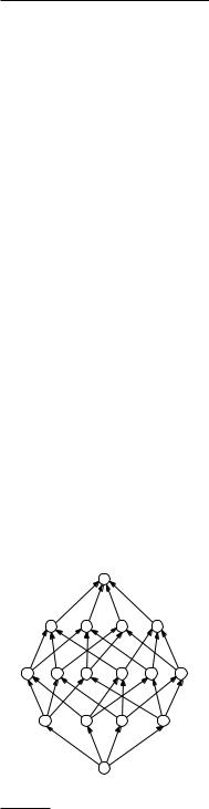
We define a directed acyclic graph G, with one source and one sink. Paths in G from the source to the sink correspond to the permutations of S. The graph G is defined as follows. There is a node for every subset of S, including one for the empty set. With a slight abuse of terminology, we shall often speak of “the subset S ” when we mean “the node corresponding to the subset S ”. It is convenient to imagine the nodes as being grouped into n + 1 layers, such that layer i contains the subsets of cardinality i. Notice that layers 0 and n both have exactly one node, which correspond to the empty set and to the set S, respectively. A node in layer i has outgoing arcs to some of the nodes in layer i + 1. More precisely, a subset S of cardinality i has outgoing arcs to the subsets S of cardinality i + 1 if and only if that S S . In other words, a subset S has an outgoing arc to a subset S if S can be obtained by adding one segment of S to S . We label the arc with this segment. Note that a subset S in layer i has exactly i incoming arcs, each labeled with a segment in S , and exactly n − i outgoing arcs, each labeled with a segment in S \S .
Directed paths from the source to the sink in G now correspond one-to-one to permutations of S, which correspond to possible executions of the algorithm TRAPEZOIDALMAP. Consider an arc of G from subset S in layer i to subset S in layer i + 1. Let the segment s be the label of the arc. The arc represents the insertion of s into the trapezoidal map of S . We mark this arc if this insertion changes the trapezoid containing point q. To be able to say something about the number of marked arcs, we use the backwards analysis argument from the

proof of Theorem 6.3: there are at most four segments that change the trapezoid containing q when they are removed from a subset S . This means that any node in G has at most four marked incoming arcs. But it is possible that a node has less than four marked incoming arcs. In that case, we simply mark some other, arbitrary incoming arcs, so that the number of marked incoming arcs is exactly four. For nodes in the first three layers, which have less than four incoming arcs, we mark all incoming arcs.
We want to analyze the expected number of steps during which the trapezoid containing q changes. In other words, we want to analyze the expected number of marked edges on a source-to-sink path in G. To this end we define the random variable Xi as follows:
1 if the i-th arc on the sink-to-source path in G is marked,
0 otherwise.
Note the similarity of the definition of Xi and the definition of Xi on page 134. The i-th arc on the path is from a node in layer i − 1 to a node in layer i, and each such arc is equally likely to be the i-th arc. Since each node in layer i has i incoming arcs, exactly four of which are marked (assuming i 4), this implies that Pr[Xi = 1] = 4/i for i 4. For i < 4 we have Pr[Xi = 1] = 1 < 4/i. Moreover, we note that the Xi are independent (unlike the random variables Xi defined on page 134).
Let Y := ∑ni=1 Xi. The number of nodes on the search path for q is at most 3Y , and we will bound the probability that Y exceeds λ ln(n + 1). We will use Markov’s inequality, which states that for any nonnegative random variable Z and any α > 0 we have
Pr[Z α ] |
E[Z] |
|
|
. |
|
α |
||
So for any t > 0 we have
Pr[Y λ ln(n + 1)] = Pr[etY etλ ln(n+1)] e−tλ ln(n+1) E[etY ].
Recall that the expected value of the sum of random variables is the sum of the expected values. In general it is not true that the expected value of a product is the product of the expected values. But for random variables that are independent it is true. Our Xi are independent, so we have
E[etY ] = E[e∑i tXi ] = E[∏etXi ] = ∏E[etXi ].
i |
i |
If we choose t = ln 1.25, we get |
|
|
|
|
|
|
|
|
|
|
|
|
|
|
|
|
|
|
||||||||
tXi |
t 4 |
0 |
|
4 |
|
|
|
|
4 |
|
4 |
|
1 |
|
1 + i |
|
||||||||||
E[e |
] e |
|
|
+ e |
(1 |
− |
|
) = (1 + 1/4) |
|
|
+ 1 − |
|
= 1 |
+ |
|
= |
|
|
, |
|||||||
i |
i |
i |
i |
i |
|
i |
||||||||||||||||||||
and we have |
|
n |
|
|
|
2 3 |
|
n + 1 |
|
|
|
|
|
|
|
|
|
|||||||||
|
|
|
|
|
|
|
|
|
|
|
|
|
|
|
|
|
|
|||||||||
|
|
|
|
∏E[etXi ] |
··· |
= n + 1. |
|
|
|
|
|
|
||||||||||||||
|
|
|
|
1 |
|
2 |
|
n |
|
|
|
|
|
|
|
|||||||||||
|
|
|
|
i=1 |
|
|
|
|
|
|
|
|
|
|
|
|
|
|
|
|
|
|
|
|
|
|
Section 6.4*
A TAIL ESTIMATE
141
Chapter 6
POINT LOCATION
142
Putting everything together, we get the bound we want to prove:
Pr[Y λ ln(n + 1)] e−λ t ln(n+1)(n + 1) = |
n + 1 |
= 1/(n + 1)λ t−1. |
|
|
|||
(n + 1)λ t |
|||
|
|
We use this lemma to prove a bound on the expected maximum query time.
Lemma 6.7 Let S be a set of n non-crossing line segments, and let λ be a parameter with λ > 0. Then the probability that the maximum length of a
search path in the structure for S computed by Algorithm TRAPEZOIDALMAP is more than 3λ ln(n + 1) is at most 2/(n + 1)λ ln 1.25−3.
Proof. We will call two query points q and q equivalent if they follow the same path through the search structure D. Partition the plane into vertical slabs by passing a vertical line through every endpoint of S. Partition every slab into trapezoids by intersecting it with all possible segments in S. This defines a decomposition of the plane into at most 2(n + 1)2 trapezoids. Any two points lying in the same trapezoid of this decomposition must be equivalent in every possible search structure for S. After all, the only comparisons made during a search are the test whether the query point lies to the left or to the right of the vertical line through a segment endpoint, and the test whether the query point lies above or below a segment.
This implies that to bound the maximum length of a search path in D, it suffices to consider the search paths of at most 2(n + 1)2 query points, one in
each of these trapezoids. By Lemma 6.6, the probability that the length of the search path for a fixed point q exceeds 3λ ln(n + 1) is at most 1/(n + 1)λ ln 1.25−1.
In the worst case, the probability that the length of the search path for any one of
the 2(n + 1)2 test points exceeds the bound is therefore at most 2(n + 1)2/(n +
1)λ ln 1.25−1.
This lemma implies that the expected maximum query time is O(log n). Take for instance λ = 20. Then the probability that the maximum length of a search path in D is more than 3λ ln(n + 1) is at most 2/(n + 1)1.4, which is less than 1/4 for n > 4. In other words, the probability that D has a good query time is at least 3/4. Similarly one can show that the probability that the size of D is O(n) is at least 3/4. We already noted that if the maximum length of a search path in the structure is O(log n), and the size is O(n), then the running time of the algorithm is O(n log n). Hence, the probability that the query time, the size, and the construction time are good is at least 1/2.
Now we can also construct a search structure that has O(log n) worst-case query time and uses O(n) space in the worst case. What we do is the following. We run Algorithm TRAPEZOIDALMAP on the set S, keeping track of the size and the maximum length of a query path of the search structure being created. As soon as the size exceeds c1n, or the depth exceeds c2 log n, for suitably chosen constants c1 and c2, we stop the algorithm, and start it again from the beginning, with a fresh random permutation. Since the probability that a permutation leads to a data structure with the desired size and depth is at least 1/4, we expect to be finished in four trials. (In fact, for large n the probability is almost one, so

the expected number of trials is only slightly larger than one.) This leads to the following result.
Theorem 6.8 Let S be a planar subdivision with n edges. There exists a point location data structure for S that uses O(n) storage and has O(log n) query time in the worst case.
The constants in this example are not very convincing—a query that visits 60 ln n nodes isn’t really so attractive. However, much better constants can be proven with the same technique.
The theorem above does not say anything about preprocessing time. Indeed, to keep track of the maximum length of a query path, we need to consider 2(n + 1)2 test points—see Lemma 6.7. It is possible to reduce this to only O(n log n) test points, which makes the expected preprocessing time O(n log2 n).
Section 6.5
NOTES AND COMMENTS
6.5 Notes and Comments
The point location problem has a long history in computational geometry. Early |
|
results are surveyed by Preparata and Shamos [323]; Snoeyink [361] gives |
|
a more recent survey. Of all the methods suggested for the problem, four |
|
basically different approaches lead to optimal O(log n) search time, O(n) storage |
|
solutions. These are the chain method by Edelsbrunner et al. [161], which is |
|
based on segment trees and fractional cascading (see also Chapter 10), the |
|
triangulation refinement method by Kirkpatrick [236], the use of persistency |
|
by Sarnak and Tarjan [336] and Cole [135], and the randomized incremental |
|
method by Mulmuley [289]. Our presentation here follows Seidel’s [345] |
|
presentation and analysis of Mulmuley’s algorithm. |
|
Quite a lot of recent research has gone into dynamic point location, where |
|
the subdivision can be modified by adding and deleting edges [41, 115, 120, 19]. |
|
A (now somewhat outdated) survey on dynamic point location is given by |
|
Chiang and Tamassia [121]. |
|
In more than two dimensions, the point location problem is still not fully |
|
resolved. A general structure for convex subdivisions in three dimensions is |
|
given by Preparata and Tamassia [324]. One can also use dynamic planar |
|
point-location structures together with persistency techniques to obtain a static |
|
three-dimensional point-location structure using O(n log n) storage and with |
|
O(log2 n) query time [361]. No structure with linear storage and O(log n) query |
|
time is known. In higher dimensions, efficient point-location structures are |
|
only known for special subdivisions, such as arrangements of hyperplanes [95, |
|
104, 131]. Considering the subdivision induced by a set H of n hyperplanes in |
|
d-dimensional space, it is well known that the combinatorial complexity of this |
|
subdivision (the number of vertices, edges, and so on) is Θ(nd ) in the worst case |
|
[158]—see also the notes and comments of Chapter 8. Chazelle and Friedman |
|
[104] have shown that such subdivisions can be stored using O(nd ) space, such |
|
that point location queries take O(log n) time. Other special subdivisions that |
|
allow for efficient point location are convex polytopes [131, 266], arrangements |
|
of triangles [59], and arrangements of algebraic varieties [102]. |
143 |
Chapter 6
POINT LOCATION
Other point location problems in 3- and higher-dimensional space that can be solved efficiently include those where assumptions on the shape of the cells are made. Two examples are rectangular subdivisions [57, 162], and so-called fat subdivisions [51, 302, 309].
Usually, a point location query aks for the label of the cell of a subdivision that contains a given query point. For point location in a convex polytope in d-dimensional space, that means that there are only two possible answers: inside the polytope, or on the outside. Therefore, one could hope for point location structures that require considerably less storage than the combinatorial complexity of the subdivision. This can be as much as Θ(n d/2 ) for convex polytopes defined by the intersection of n half-spaces [158]—see also the notes and comments of Chapter 11. Indeed, an O(n) size data structure exists in which queries take O(n1−1/ d/2 logO(1) n) time [264]. For arrangements of line segments in the plane, other implicit point location structures have been given that require less than quadratic space, even if the arrangement of line segments has quadratic complexity [7, 160].
6.6 |
Exercises |
|
|
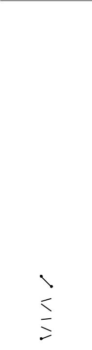
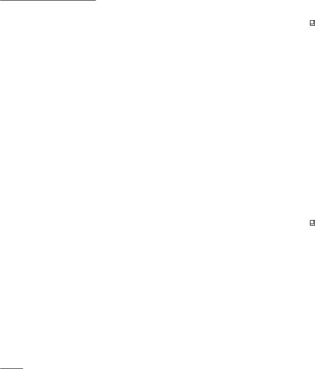
6.1 Draw the graph of the search structure D for the set of segments depicted |
|
|
|
in the margin, for some insertion order of the segments. |
|
6.2 Give an example of a set of n line segments with an order on them that |
|
|
|
makes the algorithm create a search structure of size Θ(n2) and worst-case |
|
|
query time Θ(n). |
|
6.3 In this chapter we have looked at the point location problem with pre- |
|
|
|
processing. We have not looked at the single shot problem, where the |
|
|
subdivision and the query point are given at the same time, and we have |
|
|
no special preprocessing to speed up the searches. In this exercise and |
|
|
some of the following ones, we have a look at such problems. |
|
|
Given a simple polygon P with n vertices and a query point q, here is |
|
|
an algorithm to determine whether q lies in P. Consider the ray ρ := |
|
|
{(qx + λ , qy) : λ > 0} (this is the horizontal ray starting in q and going |
|
|
rightwards). Determine for every edge e of P whether it intersects ρ . If |
|
|
the number of intersecting edges is odd, then q P, otherwise q P. |
|
|
Prove that this algorithm is correct, and explain how to deal with degen- |
|
|
erate cases. (One degenerate case is when ρ intersects an endpoint of |
|
|
an edge. Are there other special cases?) What is the running time of the |
|
|
algorithm? |
|
6.4 Show that, given a planar subdivision S with n vertices and edges and a |
|
|
|
query point q, the face of S containing q can be computed in time O(n). |
144 |
|
Assume that S is given in a doubly-connected edge list. |
6.5Given a convex polygon P as an array of its n vertices in sorted order
along the boundary. Show that, given a query point q, it can be tested in time O(log n) whether q lies inside P.
6.6Given a y-monotone polygon P as an array of its n vertices in sorted order along the boundary. Can you generalize the solution to the previous exercise to y-monotone polygons?
6.7A polygon P is called star-shaped if a point p in the interior of P exists such that, for any other point q in P, the line segment pq lies in P. Assume that such a point p is given with the star-shaped polygon P. As in the previous two exercises the vertices of P are given in sorted order along
the boundary in an array. Show that, given a query point q, it can be tested in time O(log n) whether q lies inside P. What if P is star-shaped, but the point p is not given?
6.8Design a deterministic algorithm, that is, one that doesn’t make random choices, to compute the trapezoidal map of a set of non-crossing line
segments. Use the plane sweep paradigm from Chapter 2. The worst-case running time of the algorithm should be O(n log n).
6.9* Give a randomized algorithm to compute in O(n log n + A) expected time all pairs of intersecting segments in a set of n line segments, where A is the number of intersecting pairs.
6.10Design an algorithm with running time O(n log n) for the following problem: Given a set P of n points, determine a value of ε > 0 such that the shear transformation ϕ : (x, y) →(x + ε y, y) does not change the order (in x-direction) of points with unequal x-coordinates.
6.11Let S be a set of non-crossing segments in the plane, and let s be a new segment not crossing any of the segments in S. Prove that a trapezoid ∆ of T(S) is also a trapezoid of T(S {s}) if and only if s does not intersect the interior of ∆.
6.12Prove that the number of inner nodes of the search structure D of algo-
rithm TRAPEZOIDALMAP increases by ki − 1 in iteration i, where ki is the number of new trapezoids in T(Si) (and hence the number of new leaves of D).
6.13Use a plane sweep argument to prove that the trapezoidal map of n line
segments in general position has at most 3n + 1 trapezoids. (Imagine a vertical line sweeping over the plane from left to right, stopping at all endpoints of segments. Count the number of trapezoids that are encountered by the sweep line.)
6.14We have defined the trapezoidal map of a set S of n line segments only for
the case that S is in general position. Give a definition for the trapezoidal map T(S) of an arbitrary set of segments. Prove that the upper bound of 3n + 1 for the number of trapezoids still holds.
Section 6.6
EXERCISES
p
P
145

Chapter 6
POINT LOCATION
6.15Although we have started with the point location problem on the surface of the earth, we have only treated planar point location. But the earth is a globe. How would you define a spherical subdivision—a subdivision of the surface of a sphere? Give a point location structure for such a subdivision.
6.16The ray shooting problem occurs in computer graphics (see Chapter 8). A 2-dimensional version can be given as follows: Store a set S of n
non-crossing line segments such that one can quickly answer queries of the type: “Given a query ray ρ —a ray is a half-line starting at some point—find the first segment in S intersected by ρ .” (We leave it to you to define the behavior for degenerate cases.)
In this exercise, we look at vertical ray shooting, where the query ray must be a vertical ray pointing upwards. Only the starting point need be specified in such a query.
Give a data structure for the vertical ray shooting problem for a set S of n non-crossing line segments in general position. Bound the query time and storage requirement of your data structure. What is the preprocessing time?
Can you do the same when the segments are allowed to intersect each other?
6.17* Prove a version of Theorem 6.8 that gives upper bounds for the number of nodes and the depth of the search structure without using order notation (O-bounds). The details in the text that lead to Theorem 6.8 should be modified so that it gives better constants.
146