02-03-2014_18-23-44 / A_Brief_History_of_Production_Functions

A Brief History of Production Functions

SK Mishra

Dept. of Economics

North-Eastern Hill University

Shillong (India)

Working Paper Series

Social Science Research Network (SSRN)

http://ssrn.com/abstract=1020577

Department of Economics

North-Eastern Hill University

Shillong (India)

A Brief History of Production Functions

SK Mishra

Dept. of Economics

North-Eastern Hill University

Shillong (India)

I. Introduction: Production function has been used as an important tool of economic analysis in the neoclassical tradition. It is generally believed that Philip Wicksteed (1894) was the first economist to algebraically formulate the relationship between output and inputs as P = f (x1 , x2 ,..., xm ) although there are some evidences suggesting that Johann von Thünen first formulated it in the 1840’s (Humphrey, 1997).

It is relevant to note that among others there are two leading concepts of efficiency relating to a production system: the one often called the ‘technical efficiency’ and the other called the ‘allocative efficiency’ (see Libenstein et al., 1988). The formulation of production function assumes that the engineering and managerial problems of technical efficiency have already been addressed and solved, so that analysis can focus on the problems of allocative efficiency. That is why a production function is (correctly) defined as a relationship between the maximal technically feasible output and the inputs needed to produce that output (Shephard, 1970). However, in many theoretical and most empirical studies it is loosely defined as a technical relationship between output and inputs, and the assumption that such output is maximal (and inputs minimal) is often tacit. Further, although the relationship of output with inputs is fundamentally physical, production function often uses their monetary values. The production process uses several types of inputs that cannot be aggregated in physical units. It also produces several types of output (joint production) measured in different physical units. There is an extreme view that (in a sense) all production processes produce multiple outputs (Faber, et al., 1998). One of the ways to deal with the multiple output case is to aggregate different products by assigning price weights to them. In so doing, one abstracts away from essential and inherent aspects of physical production processes, including error, entropy or waste. Moreover, production functions do not ordinarily model the business processes, whereby ignoring the role of management, of sunk cost investments and the relation of fixed overhead to variable costs (wikipedia-a).

It has been noted that although the notion of production function generally assumes that technical efficiency has been achieved, this is not true in reality. Some economists and operations research workers (Farrel, 1957; Charnes et al., 1978; Banker et al., 1984; Lovell and Schmidt, 1988; Seiford and Thrall, 1990; Emrouznejad, 2001, etc) addressed this problem by what is known as the ‘Data Envelopment Analysis’ or DEA. The advantages of DEA are: first that here one need not specify a mathematical form for the production function explicitly; it is capable of handling multiple inputs and outputs and being used with any input/output measurement; and efficiency at technical/managerial level is not presumed. It has been found useful for investigating into the hidden relationships and causes of inefficiency. Technically, it uses linear programming as a method of analysis. We do not intend to pursue this approach here.

1

Starting in the early 1950’s until the late 1970’s production function attracted many economists. During the said period a number of specifications or algebraic forms relating inputs to output were proposed, thoroughly analyzed and used for deriving various conclusions. Especially after the end of the ‘capital controversy’, search for new specification of production functions slowed down considerably. Our objective in this paper is to briefly describe that line of development. In the schema of Ragnar Frisch (1965), we will first concentrate on "single-ware" or single-output production function. Then we would move to "multi-ware" or multi-output production function. Finally, we would address the pros and cons of the aggregate production function.

II. Single Output Production Function: Humphrey (1997) gives an outline of historical development of the concept and mathematical formulation of production functions before the enunciation of Cobb-Douglas function in 1928. Paul Douglas, on a sabbatical at Amherst, asked mathematics professor Charles W. Cobb to suggest an equation describing the relationship among the time series on manufacturing output, labor input, and capital input that Douglas had assembled for the period 1889–1922, and this led to their joint paper.

An implicit formulation of production functions dates back to Turgot. In his 1767

Observations on a Paper by Saint-P´eravy, Turgot discusses how variations in factor proportions affect marginal productivities (Schumpeter, 1954). Malthus introduced the logarithmic production function (Stigler, 1952) and Barkai (1959) demonstrated how Ricardo’s quadratic production function was implicit in his tables. Ricardo used it to predict the trend of rent’s distributive share as the economy approaches the stationary state (Blaug, 1985).

Johann von Thünen was perhaps the first economist who implicitly formulated the exponential production function as P = f (F ) = A∏13 (1 − e−ai Fi ) where F1, F2 and F3 are the

three inputs, labour, capital and fertilizer, ai are the parameters and P is the agricultural production. Lloyd (1969) provides a complete account of von Thünen’s exponential production functions and their derivation. He was also the first economist to apply the differential calculus to productivity theory and perhaps the first to use Calculus to solve economic optimization problems and interpret marginal productivities essentially as partial derivatives of the production function (Blaug, 1985). Mitscherlich (1909) and Spillman (1924) rediscovered von Thünen’s exponential production function.

In The Isolated State, vol-II, von Thünen wrote down the first algebraic production function in as p = hqn , where p is output per worker (Q/L), q is capital per

worker (C/L) and h is the parameter that represents fertility of soil and efficiency of labour. The exponent n is another parameter that lies between zero and unity. Multiplying

both sides of von Thünen’s function by L (labour), we have Lp = hqn L = hC n L1−n = P =

Output. Thus, we have the Cobb-Douglas production function hidden in von Thünen’s production function (Lloyd, 1969). The credit for presenting the first Cobb-Douglas function, albeit in disguised or indirect form, must go to von Thünen in the late 1840s rather than to Douglas and Cobb in 1928 (Humphrey, 1997). Further, von Thünen was uneasy to realize the implication of his production function in which labour alone cannot

2

produce anything. Hence he modified his function to P = h(L + C)n Ln−1 . This equation,

which von Thünen estimated empirically for his own agricultural estate and which he declares he discovered only after more than 20 years of fruitless search, states that labor produces something even when unequipped with capital (Humphrey, 1997). It is surprising, however, that modern economists never formulate a production function in which labour alone can produce something.

Velupillai (1973) points out how Wicksell formulated his production function in 1900-01 that is identical to Cobb-Douglas function. In his 1923 review of Gustaf Akerman’s doctoral dissertation Realkapital und Kapitalzins, Wicksell wrote his function as with the exponents adding up to unity.

Works of Turgot, von Thünen, and Wicksell might not have been known to Paul Douglas, but it is surprising to know that before his collaboration with Cobb, Sidney Wilcox, a research assistant of Douglas, had formulated in 1926 a production function of which the Cobb-Douglas function is only a special case (Samuelson, 1979). Wilcox’s production function was, perhaps, ignored by Douglas and till date it has remained in obscurity.

Likewise, what is now well known as the Leontief production function was formulated by Jevons, Menger and Leon Walras. In the Walrasian model of general equilibrium the proportions of output to inputs are fixed and no substitution among inputs is entertained.

Bertrand Russell tells us that certain academic achievements of individual scholars are a culmination of the research efforts of an entire epoch. Such achievements are superb in exposition though containing only a little of originality, and yet they are known to the posterity by the name of those scholars in whose work they found their final expression. These achievements set forth a paradigm and thus put a halt on a further progress of science for quite a long period. This is true of Aristotle, Newton and many others (Russell, 1984: p. 521). So, it is also true of Cobb-Douglas. A notable change in his formulation of production function came only in 1961 – after a gap of 33 years – with the work of Arrow, Chenery, Minhas and Solow (1961), which, however, is only an extension, not an alternative paradigm.

Of course, two generalizations of the Cobb-Douglas production function appeared in the literature before 1961. One of them is described as P = Ae(α K / L) [K β L1−β ] and the

function only in a restricted region in the non-negative orthant of the (K, L) plane, the region in which the marginal products are nonnegative and diminishing marginal rate of substitution holds. When α > 0, 0 < β < 1 the marginal product of labour is nonnegative

only if β /α ≥ K / L . Moreover, it does not contain a linear function as its special case. The

linear production function is important in view of the Harrod-Domar fixed coefficient model of an expanding economy and therefore every neoclassical production function, the Cobb-Douglas or its generalizations, must contain the linear production function

3

to be consistent with it (Revankar, 1971). The transcendental function is a neoclassical production function if a, b < 0 and L ≤ −β / b and K ≤ −α / a (Revankar, 1971).

The transcendental function also does not contain a linear function. However, these functions allow for variable elasticity of substitution.

In the Cobb-Douglas production function the elasticity of substitution of capital for labour is fixed to unity – e.g. one percent for one percent. The production function formulated by Arrow et al. permitted it to lie between zero and infinity, but to stay fixed at that number along and across the isoquants - irrespective of the size of output or inputs (capital and labour) used in the production process. This function is well known as the Constant Elasticity of Substitution (CES) production function. It encompasses the CobbDouglas, the Leontief and the Linear production functions as its special cases.

Two mutually interrelated difficulties with the CES production function came to light very soon. The first is in the constancy of the elasticity of substitution (between inputs) along and across the isoquants and the second is in defining the said elasticity when more than two inputs are used in production. For three inputs there would be three elasticities (say, σ ij , σ ik , σ jk ) and for more inputs there would be many more. Uzawa

(1962) and McFadden (1962, 1963) proved that it is impossible to obtain a functional form for a production function that has an arbitrary set of constant elasticities of substitution if the number of inputs (factors of production) is greater than two. Mathematical enunciations of these assertions are now known as the impossibility theorems of Uzawa and McFadden.

It is rather predictable what economists would do afterwards. That is: to find a functional form of (a neoclassical) production function that would permit variable elasticities of substitution (among different inputs) along and across the isoquants as well as larger number of inputs to be included in the recipe.

m=0. For this function, the elasticity of substitution is given as σ = (1 − η + mη / Sk )−1 where

Sk is the share of capital. In 1968 Bruno formulated his Constant Marginal Share (CMS) production function P = AK α L1−α − mL or P / L = A(K / L)α − m , which implies that productivity

of labour increases with capital-labour ratio at a decreasing rate. The CMS production function contains the linear production function and defines the elasticity of substitution, σ = 1 − [mα /(1 − α )](L / P) . As the output-labour ratio increases (e.g. with economic growth),

the elasticity of substitution in this function tends to unity and thus the CMS tends to the Cobb-Douglas production function. The CMS function has nonnegative marginal productivity of labour over the entire (K, L) orthant only if m ≤ 0 (and 0 < α < 1). But then the elasticity of substitution will never be less than unity. This feature of the CMS function puts some limitation on it.

4

Lu and Fletcher (1968) generalized the CES production function to permit variable elasticity of substitution. Their “Variable Elasticity of Substitution” function is specified as P = A[δ K β + (1 − δ )η (K / L)−c(1−β ) Lβ ]1/ β . Assuming that competition has led to

(net value added). It may be noted that the assumption of minimal cost conditions and use of factor shares in defining the elasticity of substitution limit the importance of this function in empirical investigation. Ryuzo Sato and Hoffman ((1968) also introduced their variable elasticity of production function.

In his doctoral dissertation Revankar (1967) expounded his generalized production functions that permit variability to returns-to-scale as well as elasticity of substitution. In contrast with the production functions that (rather unrealistically) assume the same returns to scale at all levels of output, Zellner and Revankar (1969) found a procedure to generalize any given (neoclassical) production function with specified constant or variable elasticities of substitution such that the resulting production function retains its specification as to the elasticities of substitution all along but permits returns- to-scale to vary with the scale of output. Their Generalized Production Function (GPF) is given as where f is the basic function (e.g. Cobb-Douglas, CES, etc) as the

object of generalization, c is the constant of integration and θ , h relate to parameters

associated with the returns-to-scale function. In particular, if the Cobb-Douglas production function is generalized, we have Peθ P = AK ρα Lρ (1−α ) . This function is interesting from the viewpoint of estimation also. It has to be estimated so as to maximize the likelihood function since the Least Squares and Max Likelihood estimators of parameters do not coincide. The return to scale function is given by ρ (P) = ρ /(1 + θ P) . Depending on

the sign of θ , the returns-to-scale function monotonically increases or decreases with increase in P . However, as we know, the returns to scale first increases with output, remains more or less constant in a domain and then begins falling. This fact is not captured by the Zellner-Revankar function since it gives us a linear returns-to-scale function. Revankar (1971) presented his Variable Elasticity of Substitution (VES) production function as P = AK ρ (1−δµ ) [L + (µ − 1)K ]ρδµ with restriction on parameters:

Leontief production function (while the CES does contain it), but it contains HarrodDomar fixed coefficient model, the linear production function and the Cobb-Douglas function.

Brown and Cani (1963) had generalized the CES production to allow for nonconstant returns to scale. Nerlove (1963) had generalized the Cobb-Douglas production function to allow for variable returns to scale. Ringstad (1967) advanced on the same line. Their production function is given as P(1+c ln P ) ; c ≥ 0 , that contains the Cobb-

Douglas production function for c=0.

On the side of generalizing the CES production function to more than two factors of production, Uzawa (1962) made fundamental contributions. Further, Kazuo Sato

5

(1967) generalized the CES production function so as to incorporate more than two inputs in the recipe. To illustrate Sao’s schema, let P = f (x1 , x2 , x3 , x4 ) where P is output

and xi is an input. Now combine x1 and x2 in a manner of CES to obtain Z1 and similarly, combine x3 and x4 to obtain Z2. At the second level, combine Z1 and Z2 to obtain P. This schema would provide (constant) elasticities of substitution between x1 and x2 (say, σ12 )

and between x3 and x4 (say, σ 34 ) at the first level and between Z1 and Z2 (say, s12) at the

second level. The nesting schedule of inputs would depend on the nature of inputs and production technology.

There are ample empirical evidences that suggest capital-skill complementarity (Griliches, 1969), or the wage differential between skilled and unskilled workers. It requires two types of labour (skilled and unskilled) to be separately dealt with in specifying the production function. Obviously, the elasticity of substitution of capital for skilled labour is very little – they are complementary to each other, while the case of unskilled labour is entirely different. To specify such models, the two-level CES production technology with capital, skilled labor and unskilled labor as inputs may be more suitable.

Diewert (1971) made two very important generalizations of production functions. First, he obtained a functional form that can incorporate many inputs in the recipe and the second that such a functional form permitted variable elasticities of substitution. He generalized the Leontief production function to attain an arbitrary set of Allen-Uzawa elasticities or shadow elasticities of substitution. He also obtained the generalized linear production function that can attain an arbitrary set of direct elasticities of substitution at a given set of inputs and input prices. Diewert’s generalized linear production function is:

where h is a continuous, monotonically increasing function that tends to +∞ and has h(0)=0. Restricting the sum of coefficients to unity, this function provides convexity to the isoquants and implies a well-behaved cost function.

Griliches and Ringstad (1971), Berndt and Christensen (1973) and Christensen, Jorgenson and Lau (1973) introduced their translog production functions that permit more than two inputs as well as variable elasticities of substitution (which is a necessity in view of Uzawa-McFadden theorems). For n inputs ( xi ), the translog production

function is specified as

ln(P) = a0 + ∑in=1 ai ln(xi ) + 0.5∑in=1 ∑nj =1 bij ln(xi ) ln(x j ) ; bij = bji

Unfortunately, this function is not invariant to the units of measurement of inputs and output (Intriligator, 1978). Further, on account of inclusion of ln(xi), ln(xj), their product and their squared values, estimation of parameters of this function often suffers from multicollinearity problem.

Kadiyala (1972) proposed a production function that includes CD, CES, LuFletcher, Revankar and Sato-Hoffman production functions as its special cases. The function is defined as

6

that for ω12 = 0 his function is CES, for ω22 = 0 it is Lu-Fletcher and for ω11 = 0 it is SatoHoffman production function. He also showed that the function may be generalized for more than two inputs, but to take care of the Allen or Uzawa-McFadden partial elasticities of substitution one has to involve all the input ratios and the functional form may thus be quite lengthy and complicated. In spite of its generality, Kadiyala’s production function has remained in obscurity.

At this juncture it would be appropriate to point out that in 1967 Jan Kmenta had proposed a production function whose 2nd order Taylor’s-series approximation (around substitution parameter, β = 0 ) could be used to estimate the Constant Elasticity of

Substitution or CES production function, P = A[δ K − β + (1− δ )L− β ]-ρ/β . Kmenta obtained ln(P) = ln(A) + ρδ ln(K ) + ρ (1− δ ) ln(L) − 0.5ρβδ (1− δ )[ln(K ) − ln(L)]2 .

McCarthy (1967) pointed out that there could exist another production function

whose 2nd order Taylor’s-series approximation would be econometrically indistinguishable from Kmenta’s approximation. Thus, if one uses Kmenta’s approximation to estimate the parameters of a production function, one is not sure whether those parameters would really pertain to the CES or the McCarthy’s production function. However, enough attention has not been given to this issue, at least in the textbooks. In most cases, McCarthy’s work is ignored and unmentioned.

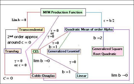
Family Tree of Linearly Homogenous Production Functions

7

Rolf Färe and Thomas Mitchell (1989) modified McCarthy’s production function by constraining a1 + a2 = 1; 0 < a1 < 1 and defining γ = a3 / b; b ≠ 0 to obtain

P = A[a1K b + (1− a1 )Lb + bγ K c Lb−c ]ρ / b

and showed that this specification, which we would call the McCarthy-Färe-Mitchell or MFM production function, has eight production functions as its special cases. A note on estimation of MFM production function is deemed necessary. It appears that if one estimates the MFM function, one can identify a variety of its special cases according to the values taken on by the estimated parameters. However, in spite of being an excellent generalization of numerous production functions, econometric estimation of MFM from empirical data is problematic due to the fact that some parameters (especially b and c) tend to be zero for some special cases. The parameter γ is a ratio (γ = a3 / b; b ≠ 0 ) and it

appears as a factor of one of the coefficients. These peculiarities may have destabilizing effect on the algorithm that estimates them.

By the middle of the 1970’s, generalization of Cobb-Douglas and CES production functions (in their classical form) was almost complete. In the classical form, these functions assume that the marginal rate of substitution between any two factors of production is associated only with relative factor prices and it is independent of technical progress or level of output or, in technical terms, the technological progress is Hicksneutral. To explain this concept a little more, we note that a technological change describes a change in the set of feasible production possibilities. A technological change is Hicks-neutral (Hicks, 1932) if the ratio of capital's marginal product to labour's marginal product is unchanged for a given capital-labour ratio. A technological change is said to be Harrod-neutral if the technology is labour-augmenting, and it is Solow-neutral if the technology is capital-augmenting. It is very easy to incorporate Hicks-neutral

does not modify the elasticity of substitution between factors of production.

Ryuzo Sato (1975) observed that so far the marginal rate of substitution function had been specified as ln(w / r) = ln(a) + (1/σ ) ln(K / L) where w and r are the prices of labour

(L) and capital (K), respectively, and σ is the elasticity of substitution. In view of the homotheticity assumption (assertion that a function g is a continuous positive monotonically increasing function of a homogenous function f, such that if y = f (x) = f (x1 , x2 ); z = g ( y) = g ( f (x)) = g ( f (x1 , x2 )) then dg / dx > 0 ) implicit in the (classical versions of) production functions (Cobb-Douglas or CES, etc. discussed so far) the marginal rate of substitution was considered to be independent of the level of production or neutral technical change. Empirical data in many cases, however, suggested that the factor price ratio varies even at a constant input ratio. An introduction of factoraugmenting technical progress (of Harrod or Solow) fails to perform due to impossibility of identification of the bias (of technical progress) and substitution effect (Sato, 1970). Therefore, Sato (1975) relaxed the homotheticity assumption so that the level of output and the degree of neutral technical progress explicitly affect the factor combinations or ln(w / r) = ln(a) + (1/σ ) ln(K / L) + b ln(P) + c ln(T (t)) , where P is the production and T(t) is the time dependent index of biased technical progress. From this specification he obtained

8

the ‘most general’ class of CES function, of which the classical CES (as well as the Cobb-Douglas) and the ‘non-homothetic Cobb-Douglas” production functions are only special cases. Sato’s generalization permitted decomposition of income and substitution effects (in the factor market) and distinction between normal and ‘inferior’ inputs.

to homotheticity (or otherwise) and separability. Since all homothetic functions are separable, Sato obtained a three-fold classification of CES. First, when dCi / df ≡ 0 and dH / df ≠ 0 , we obtain ordinary CES and Cobb-Douglas functions depending on whether

non-homogeneity parameter, we have separable non-homothetic CES function or CobbDouglas function depending on whether σ is non-unitary or unitary (Sato, 1974). In this

as well as variable elasticity of substitution. If the elasticity of substitution depends on the

isoquant but it varies across the isoquants, as output varies. It allows for a case when an isoquant in the (x1, x2) plane may be a Cobb-Douglas or (an ordinary) CES but another isoquant can be a non-homothetic CES. For n-inputs case, define for any two inputs

unitary σ respectively. In the n-inputs case we may permit variability to the elasticity of substitution across the isoquants by defining σ = σ ( f ) =constant at any f . This grand

generalization of the CES (and Cobb-Douglas) functions possibly concluded an era of investigations on this topic.

9