

Linear Engine / thesis
.pdf3.2. ELECTRICAL MACHINE SELECTION |
39 |
|||
|
|
|
|
|
|
Manufacturer |
Aerotech |
Kollmorgen |
|
|
|
|
|
|
|
Model |
BLMX-502B |
IL24-100 |
|
|
|
|
|
|
|
|
|
|
|
|
Number of Motors |
2 |
6 |
|
|
|
|
|
|
|
Peak Force (N) |
9488 |
9600 |
|
|
|
|
|
|
|
Total Cost |
$10,400 |
$19,530 |
|
|
|
|
|
|
Table 3.5: Cost Comparison by Quantity of Linear Motors
Figure 3.7: BLMX-502b Coil
larger number of lower force motors (see table 3.5 for a comparison.) Aerotech manufactures ironless linear motors at an exceptionally high force rating (other vendors, such as Kollmorgen, use a back iron design in order to achieve higher force ratings.) Aerotech’s highest force system was selected for the linear engine.
The system consisted of two each of the BLMX-502b coil (see fig. 3.7, the MTX720 magnet way (see fig. 3.8), and the BAS100 amplifier (see fig. 3.9.) Key parameters for the system are presented in table 3.6.

40 |
CHAPTER 3. DESIGN DEVELOPMENT |
Figure 3.8: MTX-720 Magnet Way
Figure 3.9: BAS-100 Sinusoidal Amplifier
3.2. ELECTRICAL MACHINE SELECTION |
41 |
||||
|
|
|
|
|
|
|
Peak Force |
4744.0 N |
|
||
|
|
|
|
|
|
|
Max Continuous RMS Force |
1186.0 N |
|
||
|
|
|
|
|
|
|
km for EMF |
54.3 |
Vpk |
|
|
|
m/s |
|
|||
|
|
|
|
||
|
km for Force |
47.4 N/Apk |
|
||
|
Internal Resistance |
1.5Ω |
|
||
|
Max Terminal Voltage |
320 V |
|
||
|
|
|
|
||
|
Coil Mass |
4.45 kg |
|
||
|
|
|
|
||
|
Coil Length |
502 mm |
|
||
|
|
|
|
||
|
Magnetic Pole Pitch |
30.0 mm |
|
||
|
Peak Amplifier Current |
100 Apk |
|
||
|
RMS Amplifier Current |
50 Apk |
|
||
|
Continuous Amplifier Power |
14.4 kW |
|
||
|
|
|
|
||
|
Amplifier Bandwidth |
2 kHz |
|
||
|
|
|
|
||
|
Total System Cost |
$15,903.00 |
|
||
Table 3.6: Key Motor System Parameters
3.2.7Verification in Simulation
Before an investment was made in the linear motor, additional simulations were conducted based on the specifications of the BLMX-502b in order to confirm that performance is acceptable. While this electrical machine is the best option within the acceptable price range for the linear motor, it was not able to meet the ideal specifications which would allow a perfectly sinusoidal piston motion profile. Therefore, three cases of nonsinusoidal trajectories which were within the capabilities of the motor were studied. The first attempts to track a sinusoid, but deviates slightly as the actuator saturates, the second was based around a wave with varying frequency, and the third demonstrates an implementation of the Atkinson cycle.
Closed Loop Simulation
In order to model actuator saturation, a closed loop controller was formulated for the linear engine. The dynamics of the system may be considered as:
42 |
CHAPTER 3. DESIGN DEVELOPMENT |
x¨ = m−1(pA − Fmot) |
(3.22) |
With Fmot as the control input, this formulation represents the entire thermodynamic system as part of the zero dynamics. Nevertheless, if one has the ability to sense pressure (which is typically the case in research engines) the trivial feedback linearizing controller,
Fmot = pA − mv |
(3.23) |
with v as the new control input, is robust to all disturbances in pressure. Further substituting v = u + x¨d to implement feed forward control, with e = x − xd, a trivial LQR controller may be designed for the error system:
e¨ = u |
(3.24) |
Yielding the overall form of the controller:
Fmot = pA − m(e · k + x¨d) |
(3.25) |
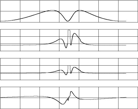
With the closed loop, actuator saturation and the resultant deviation in trajectory were simulated (see 3.10.) The deviation is only a small fraction of the total amplitude. Although this behavior is not ideal, clearly the motor can be used for a range of combustion experiments. If it is desirable to more closely approximate crankshaft behavior, a future generation of the linear engine could use four rather than two linear motors.
Variable Rate
This simulation expanded upon the closed loop system described above. But, instead of a regular sinusoid, the system is driven with a frequency modulated sine wave (see

3.2. ELECTRICAL MACHINE SELECTION |
43 |
|
0.2 |
|
|
|
|
|
|
|
|
|
(m) |
|
|
|
|
|
|
|
|
|
|
position |
0.1 |
|
|
|
|
|
|
|
|
|
|
|
|
|
|
|
|
|
|
|
|
|
0 |
0 |
|
0.02 |
0.04 |
0.06 |
0.08 |
0.1 |
0.12 |
0.14 |
|
|
4 |
||||||||
(N) |
1 |
x 10 |
|
|
|
time (s) |
|
|
|
|
|
|
|
|
|
|
|
|
|
||
force |
|
|
|
|
|
|
|
|
|
|
|
|
|
|
|
|
|
|
|
|
|
motor |
0 |
|
|
|
|
|
|
|
|
|
|
|
|
|
|
|
|
|
|
|
|
linear |
−1 |
0 |
|
0.02 |
0.04 |
0.06 time (s) |
0.08 |
0.1 |
0.12 |
0.14 |
|
|
|||||||||
(A) |
100 |
|
|
Irms=59.646 A, Ipk=100.13 A |
|
|
|
|
|
|
|
|
|
|
|
|
|
|
|||
current |
0 |
|
|
|
|
|
|
|
|
|
|
|
|
|
|
|
|
|
|
|
|
−100 |
0 |
|
0.02 |
0.04 |
0.06 |
0.08 |
0.1 |
0.12 |
0.14 |
|
|
|
|
||||||||
(V) |
500 |
|
|
time (s) |
|
|
|
|
voltage |
|
Vpk=306.68 V |
|
|
|
|
|
|
0 |
|
|
|
|
|
|
|
|
−500 |
|
|
|
|
|
|
|
|
terminal |
0 |
0.02 |
0.04 |
0.06 time (s) |
0.08 |
0.1 |
0.12 |
0.14 |
|
||||||||
Figure 3.10: Mechanical and Electrical Data for Closed Loop Simulation

44 |
CHAPTER 3. DESIGN DEVELOPMENT |
|
x 10 |
6 |
p V plot |
|
|
|
6 |
|
|
|
|
|
5 |
|
|
|
|
|
4 |
|
Ideal |
|
|
|
|
|
|
|
|
|
|
|
Closed Loop |
|
|
(pa) |
|
|
|
|
|
pressure |
3 |
|
|
|
|
|
|
|
|
|
|
|
2 |
|
|
|
|
|
1 |
|
|
|
|
|
0 |
2 |
4 |
6 |
8 |
|
0 |
||||
|
|
|
volume (m3) |
|
x 10−4 |
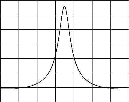
Figure 3.11: PV Diagram for Closed Loop Simulation
3.2. ELECTRICAL MACHINE SELECTION |
45 |
|
|
0.2 |
|
|
|
|
|
|
|
(m) |
|
|
|
|
|
|
|
|
|
position |
0.1 |
|
|
|
|
|
|
|
|
|
|
|
|
|
|
|
|
||
|
|
0 |
0.05 |
0.1 |
0.15 |
0.2 |
0.25 |
0.3 |
0.35 |
(N) |
|
0 |
|||||||
|
|
|
|
|
time (s) |
|
|
|
|
|
|
|
|
|
|
|
|
|
|
10000 |
|
|
|
|
|
|
|
||
force |
5000 |
|
|
|
|
|
|
|
|
motor |
|
0 |
|
|
|
|
|
|
|
|
|
|
|
|
|
|
|
|
|
−5000 |
0.05 |
0.1 |
0.15 |
0.2 |
0.25 |
0.3 |
0.35 |
||
linear |
|
0 |
|||||||
|
|
200 |
|
|
|
time (s) |
|
|
|
|
|
|
|
|
|
|
|
|
|
|
(A) |
100 |
|
|
|
|
|
|
|
|
current |
Irms=23.473 A, Ipk=100.13 A |
|
|
|
|
|
||
|
0 |
|
|
|
|
|
|||
|
|
|
|
|
|
|
|
||
|
|
|
|
|
|
|
|
|
|
|
−100 |
0.05 |
0.1 |
0.15 |
time (s) |
0.25 |
0.3 |
0.35 |
|
|
|
0 |
0.2 |
||||||
(V) |
500 |
|
|
|
|
|
|
|
|
voltage |
0 |
Vpk=302.04 V |
|
|
|
|
|
|
|
|
|
|
|
|
|
|
|
||
−500 |
|
|
|
|
|
|
|
|
|
terminal |
0 |
0.05 |
0.1 |
0.15 |
time (s) |
0.2 |
0.25 |
0.3 |
0.35 |
|
|||||||||
Figure 3.12: Mechanical and Electrical Data for Variable Rate Simulation
fig. 3.12.) The frequency modulation is tuned to increase the rate of acceleration during the expansion stroke in order to reduce the peak force. Then, during intake and exhaust when the piston speed is less critical, the system slows down significantly in order to reduce the RMS force. This motion profile can be sustained by the linear motor indefinitely and results in minor changes to the PV diagram such as a slight decrease in peak pressure (see fig. 3.13.)

46 |
CHAPTER 3. DESIGN DEVELOPMENT |
|
x 10 |
6 |
p V plot |
|
|
|
6 |
|
|
|
|
|
|
|
|
|
Ideal |
|
|
|
|
|
Variable Rate |
|
5 |
|
|
|
|
|
4 |
|
|
|
|
(pa) |
|
|
|
|
|
pressure |
3 |
|
|
|
|
|
|
|
|
|
|
|
2 |
|
|
|
|
|
1 |
|
|
|
|
|
0 |
2 |
4 |
6 |
8 |
|
0 |
||||
|
|
|
volume (m3) |
|
x 10−4 |
Figure 3.13: PV Diagram for Variable Rate Simulation
3.2. ELECTRICAL MACHINE SELECTION |
47 |
Equivalent Rotational Speed vs. Time
|
1400 |
|
|
|
|
|
|
|
|
1200 |
|
|
|
|
|
|
|
Speed (RPM) |
1000 |
|
|
|
|
|
|
|
800 |
|
|
|
|
|
|
|
|
Rotational |
600 |
|
|
|
|
|
|
|
Equivalent |
400 |
|
|
|
|
|
|
|
|
|
|
|
|
|
|
|
|
|
200 |
|
|
|
|
|
|
|
|
0 |
0.05 |
0.1 |
0.15 |
0.2 |
0.25 |
0.3 |
0.35 |
|
0 |
Time (s)
Figure 3.14: Equivalent Crankshaft Speed
48 |
CHAPTER 3. DESIGN DEVELOPMENT |
Atkinson
As discussed in chapter 1, the ability to implement the Atkinson cycle is an important advantage to employing piston motion profiles unconstrained by a traditional crankshaft. Additional energy is extracted by lengthening the expansion stroke until the cylinder pressure at bottom dead center is near the ambient pressure. A simulation demonstrating the linear engine’s ability to implement the Atkinson cycle was carried out by amplitude modulating a sinusoid to create an asymmetric desired trajectory for the piston motion (see fig. 3.15.) Other than the modified command signal, the simulation was carried out as in the first closed loop case described above.
Because of the higher peak velocity due to the larger amplitude in part of the sinusoid, the equivalent rotational speed had to be reduced to 700 RPM in order to avoid exceeding the maximum coil voltage. This lower speed led to slightly greater deviation from the desired trajectory during the combustion event than occurred in the other simulations. For comparison, a simulation was run with a pure sinusoidal motion profile under similar conditions (see fig. 3.16 for the PV diagrams.) The pressure does not quite reach ambient, but extending the expansion stroke further would have yielded diminishing returns in recovered energy while further taxing the velocity and force capabilities of the linear motor. In this simulation, the Atkinson trajectory extracted 6.3% more work then the pure sinusoidal trajectory.
3.3Linear Motor Prototype
The next step was to prototype the operation of the linear motor. The purpose of the prototype was to learn how to apply the technology, while establishing basic function. Additionally, the prototyping process served to verify key assumptions and parameters about the motor. These goals engendered several requirements of the prototype structure. The magnet way needed to be kept stationary, and the prototype