1.5 Похибки прямих вимірювань Похибки прямих вимірювань визначаються за формулою

, n = 1, (1.18)

якщо деяку величину виміряти один раз.

Якщо вимірювання виконувались n раз , то

, n > 1. (1.19)

В цих рівняннях t_∞ - коефіцієнт Стьюдента для заданого  при необмеженому числі вимірів;  - похибка приладу; ν - похибка відліку, .

Наприклад: довжина тіла була виміряна 3 рази:

n	х, мм	∆хi , мм	(Δхi)²
1	12,8	0,446	0,217
2	13,6	0,334	0,111
3	13,4	0,134	0,018
=13,2		∑(Δхi)²=0,3

Відносна похибка дорівнює

.

Кінцевий результат: x = (13,3 ± 0,3) мм ; α = 0,7 ; Е = 3,6 %.

1.6 Похибки непрямих вимірювань

Якщо y - величина, що вимірюється посередньо, її розраховують за відомою залежністю y=f(x₁,x₂,…x_n) від змінних x₁,x₂,,…x_n, які вимірюють безпосередньо.

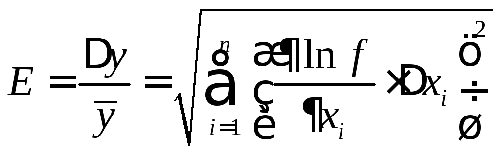
1. Похибки непрямих вимірів визначаються за формулою:

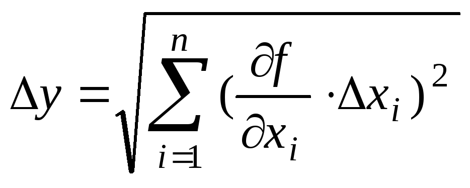, (1.20)

якщо функціональна залежність досліджуваної величини є багаточлен.

2. Похибки непрямих вимірів можна визначати

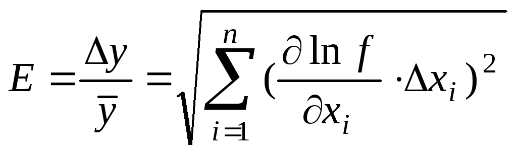, (1.21)

.

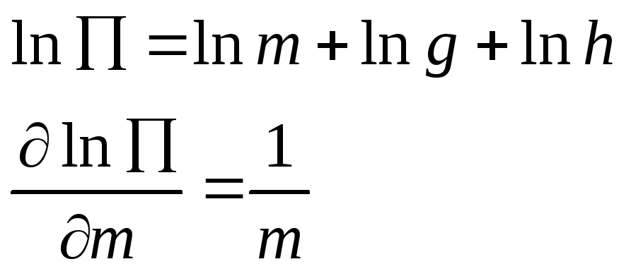
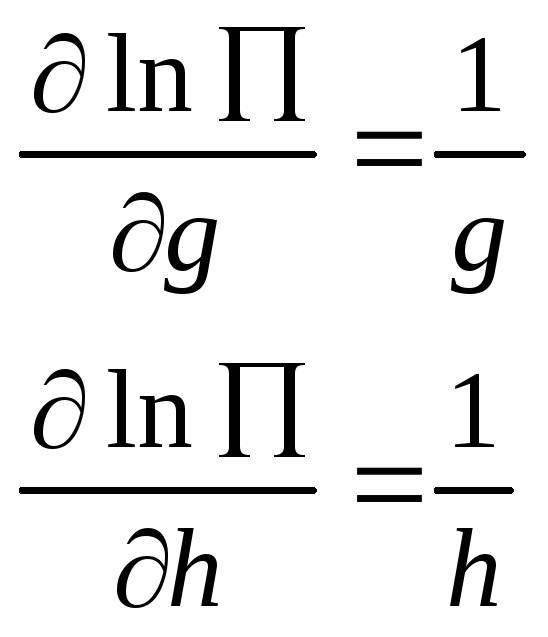
якщо функціональна залежність досліджуваної величини є одночлен і потім знаходимо y як: . Наприклад:

1. Якщо залежність функції , тоді

Тоді

.

2. Якщо залежність функції: ,

Тоді

,

.

У результаті отримуємо

.

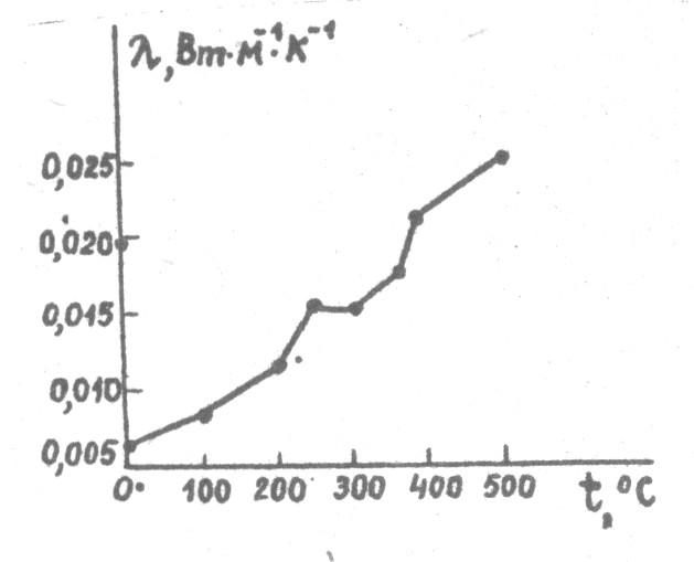
1.7 Графічне відображення експериментальних результатів

Графік будується на міліметровому папері. На рисунках нижче можна побачити приклади графіків.

невірно вірно

Експериментальна крива проходить крізь експериментальні точки.

Контрольні запитання

1. Дати визначення прямих і непрямих вимірів. Приклади.

2. За допомогою якої формули знаходять найбільш ймовірне значення виміряної величини?

3. Що таке відносна похибка?

4. Що називається випадковим відхиленням?

5. За якою формулою знаходять середнє квадратичне значення або похибку, викликану випадковими відхиленнями?

6. За якою формулою знаходять похибки засобів виміру.

7. За якою формулою знаходять похибки табличних величин та відліку.

8. Сформулюйте правила округлення.

9. Запишіть формули обчислення похибок при прямих вимірах.

10. Запишіть формули обчислення похибок при непрямих вимірах.

Рекомендована література

1. Методичні вказівки до лабораторних занять з механіки та молекулярної фізики.- Запоріжжя: ЗНТУ, 2003.–С.7-17.- 60 с.

Доповнення і редагування:

доцент кафедри фізики, канд. фіз.-матем. наук В. Г. Корніч;

професор кафедри фізики, д-р. фіз.-матем. наук С. В. Лоскутов.

Затверджено на засіданні кафедри фізики ЗНТУ, протокол № 3 від 01.12.2008 р.

2 ELEMENTS OF THE THEORY OF ERRORS

Measurement of physical quantities means their comparison with standard. There are two types of physical measurements:

1. Direct measurements are measurements when the investigated quantity x is taken by direct comparison with the standard performed with instruments.

2. Indirect measurements consist of direct measurements of physical quantities x₁, x₂,.., x_n and calculations made on this basis the investigated quantity y by a functional dependency y = f(x_1, x₂ ,...,x_n ).

For example: measurements of length by a ruler or measurements of temperature with a thermometer are direct measurements. But measurement of volume of a cylinder by the value of its height h and diameter d (these are direct measurements) with functional relation V=d²h/4 is an indirect measurement.

All measurements can be performed only up to a certain degree of precision. Error of measurements is defined as a deviation of the result of measurements from the true value of a measured quantity.

Then, by definition

,

where x is absolute error of x measures.

The problems of the Theory of Errors are:

1. To get the investigated quantity.

2. To get the error of measurements.

There are two kinds of measurements errors: systematic errors and accidental ones.

Systematic error is defined as a component of error; its quantity is constant in all measurements or is being regularly changed during the repeated measurements of the physical quantity.

Accidental error is defined as a component of error that is changed irregularly during repeated measurements of the same physical quantity.

One should distinguish between blunder and above mentioned errors. Its value is essentially greater than the expected error in given conditions. For example, these errors may be received if an instrument is faulty, or if an experimenter is inattentive and so on.

2.1 Principal concepts of the theory of errors

We can't define the true values of a physical quantity. We can define only the interval (x_min , x_max) of the investigated quantity with some probability . For example: we can affirm, that students' height may be defined between 1.5 m and 2.0 m with probability of 0.9. Then we can prove, that students' height may be defined between 1.6 m and 1.8 m with smaller probability of 0.6 and so on. Value of this interval is called the entrusting interval. On fig.2.1 interval of quantity being investigated x is represented.

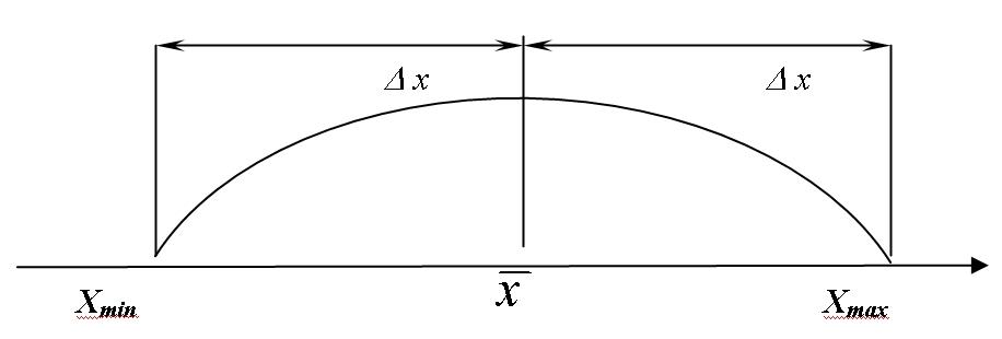
Figure 2.1

Where x is the most probable value of quantity being measured; x is the half width of the entrusting interval of the measured quantity with probability of .

Therefore we can estimate, that true value of the measured quantity may be defined as x = x  x, with probability ,

or .

If a quantity x has been measured n times and x₁ , x₂ ,..., x_n are the results of the individual measurements then the most probable measured value or the arithmetic mean is:

(2.1)

The deviation is called the accidental error (deviation) of a single measurement.

(2.2)

is called the mean accidental deviation of the measurements.

Mean root square is defined as

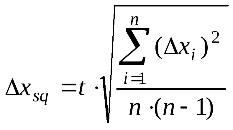(2.3)

where t – Student’s constant for definite  and n. The ratio of

(2.4)

is called the relative error of measurement and is usually expressed in percents:

. (2.5)

2.2 Errors of instruments

Absolute error of instrumental  is a deviation

, (2.6)

where a is an index of an instrument; X is the true value of the quantity measured. Typically  is quantity of the instruments minimum value scale. For example: the ruler error is  = 1 mm.

Relative error of the measurement is the ratio of

. (2.7)

It is usually expressed in percent

. (2.8)

Brought error of the measurement or precision class is the ratio

, (2.9)

expressed in percent. D is maximum value on the instrument scale.

For example: electric current is measured by the instrument with interval 0 ÷ 1 A, precision class is 0.5. This means, that D = 1 A,  = 0.5 %, and

.

If the instrument shows 0.3 A, then

.

2.3 Error of table quantities, count and rules of approximations

1. The error of table quantity is defined as

, (2.10)

where, α is probability; v is half price of category from last significance figure in table quantity. For example: quantity  may be 3.14. In this case v = 0.005 and

.

If quantity  is 3.141 and v = 0.0005 then

and so on.

2. Error of count may occur when we measure quantity by an instrument. Typically, the error of count is half price of minimum value of instruments scale. For example a ruler has error of count v_l=0.5 mm.

3. Rules of approximation: quantity x may be approximated only to two significant figures, if the first significant figure is 1 or 2. In other cases, the quantity is approximated only to one significant figure. For example: x = 0.01865, approximated quantity is 0.019; x = 0.896, approximated quantity is 0.9 and so on.

2.4 Errors of direct measurement

Errors of direct measurements are defined as

, (2.11)

if there is one measurement (n = 1). And

, (2.12)

if there are several measurements (n > 1).

In these equations t_ is Student's constant, it may be defined from the table on the crossing of line with n and column with ;  is error of an instrument; v is error of count, v =/2.

For example: the length of a body was measured three times:

xi, mm	xi, mm	(xi)2, mm2
12.8	-0.466	0.217
13.6	0.334	0.111
13.4	0.134	0.018
=13.266, n=3, t=1.4, t=1, =1 mm.

The error of this measurement will be:

The relative error is

.

The final result is

x = (13.3 + 0.5) mm, = 0.7 , E = 3.6 % .

2.5 Errors of indirect measurements

Let y be indirectly measured quantity, it is defined as y = f(x₁ ,x₂ , ..., x_n ). x₁ ,x₂ , ... , x_n is defined as the direct measurements.

1. Errors of indirect measurements are defined as

(2.13)

if the functional dependence of investigated quantity is a polynomial.

2. Errors of indirect measurements are defined as

(2.14)

if the functional dependence of investigated quantity, is a monomial

and we can define y as: . For example:

1. If the functional dependence is then

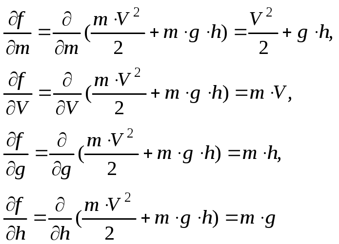
Then

2. If functional dependence is ,

Then

and

The final result: .

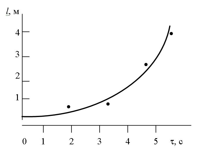
2.6 Graph presentation of the experimental results

Graph is built on the millimeter paper. In fig.2.2 you can see an example of graph.

Figure 2.2

The experimental curve is drawn through the experimental points. This curve describes the experimental data.

Control questions

1. Definition of direct and indirect measurements. Examples.

2. Definition of the most probable value of the measured quantity x.

3. What is called a relative error?

4. What is called an accidental deviation?

5. What is the equation of square mean of errors?

6. How do we define errors of instruments?

7. How do we define errors of table quantities and count errors?

8. Rules of approximation.

9. What is the equation of errors of direct measurements?

10. What is the equation of errors of indirect measurements?

Authors: S.P. Lushchin, the reader, candidate of physical and mathematical sciences.

Reviewer: S.V. Loskutov, professor, doctor of physical and mathematical sciences.

Approved by the chair of physics. Protocol № 3 from 01.12.2008 .