5.1 Convolutional Filters

Listing 5.1 presents the general structure of a convolutional filter. Any convolutional filter is defined by means of the values of the mask m , with the (odd) side of the mask, provided these values are held constant regardless the coordinate they are applied to and the values of the input image f. We say that g = f ∗ m is the result of applying to f the convolution filter defined by the mask m when the output image is defined by

gf), (5.1)

for every (i, j). This operation consists in overlaying the mask on each coordinate of f, making the product of each value in the mask with the corresponding value in the image, and then adding all the products to compute the corresponding value in the output image g. R performs this in a rather economicway; in fact, f[(i-km1d2):(i+km1d2),(j-km1d2):(j+km1d2)] (line 15 ofListing 5.1) captures all the required values in the input image f. Then* m(line 16) performs the pointwise product of these values with those in the mask m. Finally, the command sum returns the sum of all these products.

The result will depend only on the definition of the values in the mask. There are many ways to specify masks depending on the desired output. The reader isreferred to the book by Goudail and Réfrégier (2003) for a comprehensive account of approaches. Particular maskswill be denoted by the capital letter M with amnemonic subscript. The identity mask M1, defined as m00 = 1 and zero elsewhere, produces

a copy of f, i.e., f = f ∗ M1.

If all the entries of the mask are nonnegative, the filter is usually called “lowpass” because, when analyzed in the frequency domain, any filter of this class will reduce the high-frequency content (mainly due to noise and abrupt changes as, for instance, edges and small features) enhancing the low-frequency component (which is associated to flat or slowly varying areas). The books by Jain (1989) and Lim (1989) are excellent references for the analysis of images in the frequency domain, of which we will only borrow some terminology. In the following we will see the effect of a number of low-pass filters.

The first class of low-pass filters we will analyze is formed by those which consist of computing the mean using a some or all the elements of the mask. Consider the following masks:

5.1Convolutional Filtres

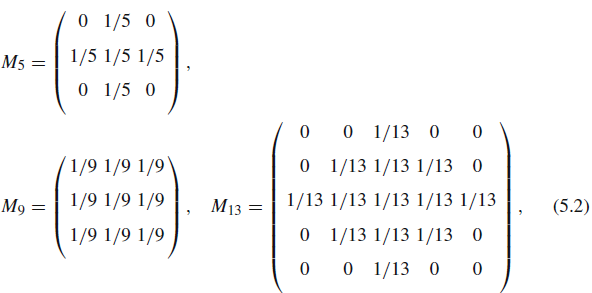
M₁₂₁ = (1/121) in every − 5 ≤ i, j ≤ 5. (5.3)

They all add up to 1, a very convenient normalization in light of the following result.

Claim (The mean value of images filtered by convolution) Let f be an image such that its mean value is finite, and m a finite mask conveying finite values. The mean value of g = f ∗ m is the product of the mean values of f and of m.

Since more often than not we will be working with images defined on a compact set of values K, the unitary cube [0,1]³ for instance, this result allows us to transform f into g, whose values are not too far from K.

They all add up to 1, a very convenient normalization in light of the following result.

Claim (The mean value of images filtered by convolution) Let f be an image such that its mean value is finite, and m a finite mask conveying finite values. The mean value of g = f ∗ m is the product of the mean values of f and of m.

Since more often than not we will be working with images defined on a compact set of values K, the unitary cube [0,1]³ for instance, this result allows us to transform f into g, whose values are not too far from K.

Listing 5.2 shows how to create the masks and the use of the ConvolutionFilter function already defined in Listing 5.1.

Listing 5.2 Building masks and applying mean filters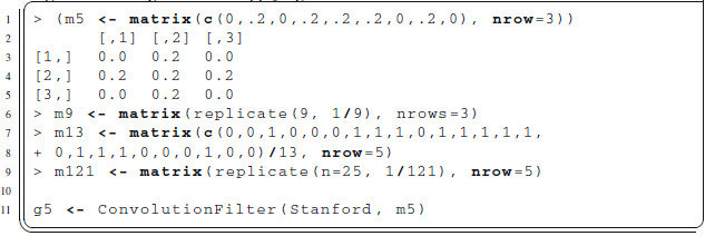

Figure5.2 shows the result of applying the masks defined in Eqs.(5.2) and (5.3) The blurring effect in the first three is subtle, and becomes evident in the last one.

Figure5.3 shows the profile of the original and filtered images restricted to the vertical strips. Notice the smoothing effect which consists in reducing the width of the peak, up to the point of almost eliminating the variability when the M₁₂₁ mask is applied. The mean value, as expected, is preserved. Notice also that the characters become almost solid, but heavily blurred. The untouched region close to the edges is noticeable in this last example.

1. (b)

Fig. 5.2 Results of applying mean filters to the original image. a f ∗ M₅. b f ∗ M₉. c f ∗ M₁₃. d f ∗ M₁₂₁

Convolution is quite general and is not limited to equal values, as considered so far. Besides the mean filter, another important low-pass convolution filter is the Gaussian mask. A Gaussian mask of side and standard deviation σ is defined by first computing

m, (5.4)

2 and then using the normalized mask m = m , . These values decrease exponentially fast from the center to the edges of the mask. Gaussian convolution filters are at the core of multilevel techniques (Medeiros et al. 2010).

Listing 5.3 presents the code that returns the Gaussian mask of side side and standard deviation s. Lines 3–5 define the auxiliary function DExp; it was defined withinthescopeofGaussianMaskinordertomakeitawareoftheinputparameter s since, as required later, it has to have as arguments the two variables that will comprise the grid. This auxiliary function implements Eq.(5.4).

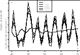Fig. 5.3 Strips profiles at line 240

Column

Listing 5.3 Building a Gaussian mask

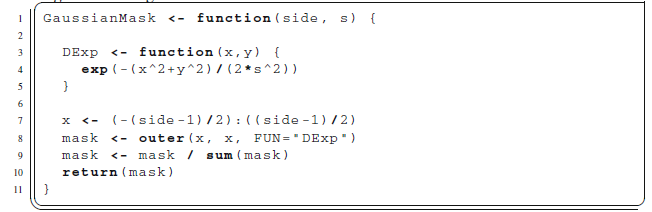
Line 7 builds one of the variables that will define the support of the mask, say i. There is no need to build the other variable (j) since they are equal: -(l-1)/2>=i ,j<=(l-1)/2. The function outer used in line 8 takes as input two vectors (the same in our case) and returns a grid whose values are the result of instantiating the function DExp in each of all the possible pairs of values of the input vectors. Line 9 normalizes the result in order to make the sum one.

The following code illustrates three examples of Gaussian masks as computed by the function presented in Listing 5.3, all of them of side five with varying standard deviations. Notice that when σ → 0 the Gaussian mask converges to the identity mask, while when σ → ∞ it becomes the mean over all the elements of the mask.

> (GaussianMask(5,.5))

[,1] [,2] [,3] [,4] [,5]

[1,] 7.0e-08 2.8e-05 0.00021 2.8e-05 7.0e-08

[2,] 2.8e-05 1.1e-02 0.08373 1.1e-02 2.8e-05

[3,] 2.1e-04 8.4e-02 0.61869 8.4e-02 2.1e-04

[4,] 2.8e-05 1.1e-02 0.08373 1.1e-02 2.8e-05

[5,] 7.0e-08 2.8e-05 0.00021 2.8e-05 7.0e-08 > (GaussianMask(5,1))

[,1] [,2] [,3] [,4] [,5] [1,] 0.003 0.013 0.022 0.013 0.003

[2,] 0.013 0.060 0.098 0.060 0.013

[3,] 0.022 0.098 0.162 0.098 0.022

[4,] 0.013 0.060 0.098 0.060 0.013

[5,] 0.003 0.013 0.022 0.013 0.003 > (GaussianMask(5,10))

[,1] [,2] [,3] [,4] [,5] [1,] 0.039 0.040 0.040 0.040 0.039

[2,] 0.040 0.040 0.041 0.040 0.040

[3,] 0.040 0.041 0.041 0.041 0.040

[4,] 0.040 0.040 0.041 0.040 0.040

[5,] 0.039 0.040 0.040 0.040 0.039

Figure5.4 shows the result of applying two Gaussian filters with the same window

5) and two different values of standard variation: Figure5.4a is the result for σ = 1, while Fig.5.4b is the result for σ = 10. The difference is noticeable: the latter is more blurred than the former.

Somewhere between the mean filters, which has binary coefficients, and the Gaussian filter, whose values decay exponentially with the Euclidean distance to the center of the mask, there is the binomial filter. The binomial mask is defined as the product of all the binomial coefficients C, where is even (so the vector and the mask are odd) and 0.

The code presented in Listing 5.4 shows how to compute this masks in R using the choose function, the product of vectors (and matrices) \%*\%, and the transpose

(a) (b)

Fig. 5.4 Results of applying the Gaussian filter of side5 and varyingσ. aσ = 1. b σ = 10

operator t. The values are shown before dividing by the sum of the mask, but the operation commented in line 4 must be activated when building binomial masks.

Listing 5.4 Building a biominal mask

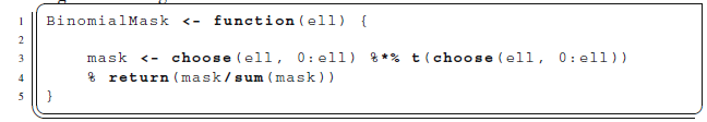
A few binomial masks are shown in the following.

> BinomialMask(4)

[,1] [,2] [,3] [,4] [,5]

[1,] 1 4 6 4 1

[2,] 4 16 24 16 4

[3,] 6 24 36 24 6

[4,] 4 16 24 16 4

[5,] 1 4 6 4 1

> BinomialMask(6)

[,1] [,2] [,3] [,4] [,5] [,6] [,7]

[1,] 1 6 15 20 15 6 1

[2,] 6 36 90 120 90 36 6

[3,] 15 90 225 300 225 90 15

[4,] 20 120 300 400 300 120 20

[5,] 15 90 225 300 225 90 15

[6,] 6 36 90 120 90 36 6

[7,] 1 6 15 20 15 6 1

> BinomialMask(8)

[,1] [,2] [,3] [,4] [,5] [,6] [,7] [,8] [,9]

[1,] 1 8 28 56 70 56 28 8 1

[2,] 8 64 224 448 560 448 224 64 8

[3,] 28 224 784 1568 1960 1568 784 224 28

[4,] 56 448 1568 3136 3920 3136 1568 448 56

[5,] 70 560 1960 3920 4900 3920 1960 560 70

[6,] 56 448 1568 3136 3920 3136 1568 448 56

[7,] 28 224 784 1568 1960 1568 784 224 28

[8,] 8 64 224 448 560 448 224 64 8

[9,] 1 8 28 56 70 56 28 8 1

Figure5.5 presents the results of applying the binomial masks of sides 7 and 13 to the input image. Notice that the contrast is reduced in the second with respect to the first due to the extent of the mask; it “mixes” the values and both pure black and white tend to disappear.

(a) ()

Fig. 5.5 Result of applying the binomial masks. a Binomial filter of side 7. b Binomial filter of side 13

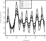Fig. 5.6 Strips profiles at line 80

Figure5.6 presents the profile of line 80 at the strips (columns 30–70) of the original image, and of the images filtered by the Gaussian (with σ = 1 and σ = 10) and by the Binomial (of sides 7 and 13) masks.

So far we have seen low-pass filters, i.e., those defined by nonnegative values of the filter mask. In the following we will see an important application of high-pass filters, namely edge detection. This will require the use of negative values.

The first class of high-pass filters we will describe is known as unsharp masking. The idea is to enhance the rapid variations in the image, which correspond to edges and sharp transitions, by subtracting a fraction α, 0 < α < 1, of an smoothed version Υ( f ) of the original image to the original image f. The result is |(1−α) f +αΥ( f )|, conveniently scaled to the [0,1] range.

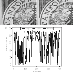
Fig. 5.7 Edge enhancement by unsharp masking with α = 3/10. a Mean with the M₁₂₁ mask. b Binomial filter of side 17. c Profiles at line 80

Figure5.7presentstheresultsofapplyingtheunsharpmaskingtechniquewithtwo different blurred images and the same value of α = 3/10. Figure5.7a was obtained applying the mask defined in Eq.(5.3), i.e., a 11 × 11 mask of ones, while Fig.5.7b shows the result of applying the binomial mask of side 17. Albeit the difference between the masks, the results are alike. This powerful technique requires trial-anderror until the desired result is obtained.

Figure5.7c shows the profile of the original and transformed images. Notice how relatively flat (smooth) areas had their values reduced, while sharp transitions are left unaltered. This transformation leads to a perceptual edge enhancement.

Fig. 5.8 Using the Laplacian mask. a Image filtered with the Laplacian mask. b Image enhanced with the Laplacian mask. c Profiles at line 80

As previously said, oftentimes it is desirable to enhance edges and sharp transitions.

If we envision the image f : S → R as the discrete version of a continuous function f : R² → R. Those features could be detected in f by applying the gradient operator

∇ = (∂/∂x,∂/∂y), but since we do not possess the analytic (functional) description of f , a discrete version of ∇ could be applied to f instead. This can be performed

by convolving the original image with the Laplacian mask:

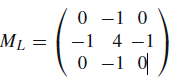(5.5)

5.1 Convolutional Filters

The edges detected by the Laplacian mask are shown in Fig.5.8a. They can be used to enhance the original image by adding the filtered version to it. Replacing the value 4 by 5 in Eq.(5.5) does the trick, and produces the image shown in Fig.5.8b. Figure5.8c presents the profiles of the original and enhanced images at line 80. We notice the same effect already described in the unsharp masking technique: a reduction of smoothly varying areas. The Laplacian filter tends to produce noisy images, since it enhances every little variation, even those due to noise.