

Chapter 5
Filters in the Image Domain
Filtro de Amor: 20 vellos tuyos, 3 gramos de polvo de tus uñas, o tres gotas de tu sangre (imprescindible; es la clave del filtro de amor, sirve para que el efecto de amor del filtro vaya dirigido hacia ti). http://www.tarot-amor-gratis.com/filtro_amor.htm
In this chapter we will see how to build filters defined on the image domain. They all share the property of being functions of values around the pixel being processed, so we will not consider approaches based on transformations as, for instance, Fourier or Wavelet domain. Albeit limited, this approach will allow the user to build and experiment with image filters. A more model-based approach can be found in the book by Velhoet al. (2008). Other important references are the works by Barrett and Myers (2004); Jain (1989); Lim (1989); Lira Chávez (2010); Gonzalez and Woods (1992); Myler and Weeks (1993); Russ (1998) among many others.
The reader is invited to recall the definitions of local operations, neighborhood and mask presented in Chap.1(p. x and 6). All the filters we consider will be defined on a mask: iff is the input image, then g = ΥM( f ) is the result of applying the filter Υ with respect to the mask M to f . Each element of g is a function of the values observed in f locally with respect to the mask M and the values it conveys. For the sake of simplicity, all considered masks will be of the form presented in Eq.(2.3):
M × ,
i.e.,
masks are squared sets of coordinates of (odd) side . Oftentimes, we
will need to define values in each mask coordinate, i.e., we will
work with matrices of the form
![]() .
The term “mask” and the notationM
will
be employed for both the support and the values.
.
The term “mask” and the notationM
will
be employed for both the support and the values.
For the sake of simplicity, in all the theoretical descriptions we will assume that the input and output images are defined on the infinite support S = Z2. When implementingthefilters,thefinitenatureoftheimagesneedstobetakenintoaccount. This can be done in at least two ways, namely, modifying the mask whenever needed
A. C. Frery and T. Perciano, Introduction to Image Processing Using R,59
SpringerBriefs in Computer Science, DOI: 10.1007/978-1-4471-4950_7_5,
© Alejandro C. Frery 2013
(close to the edges of the original image), or applying the transformation only to those coordinates where the mask fits in. The latter will be used in our examples, as illustrated in the following code that will be common to all filters here discussed.
Listing 5.1 presents the general convolution filter. It takes two arguments as input, the image to be filtered and the mask. The first operations consist in discovering the number of lines and columns of the original image (lines 6 and 7, respectively), and the side of the mask (line 8). Line 10 creates the container for the output image g by copying the input image f; g is created with the dimensions, type, and additional attributes f has.
Listing 5.1 Convolution filter
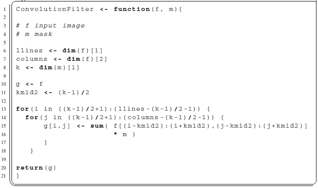
Assume f has m lines and n columns, and that it will be filtered by a mask of (even) side k. If we choose to filter only those pixels over which the mask fits, then our filter must start in line and column (k − 1)/2 + 1, and stop in line m −(k − 1)/2 − 1 and column n −(k −1)/2−1. Listing 5.1 performs this in lines 13 and 14; please notice the use of parenthesis, they are mandatory due to the operations precedence. Lines 15 and 16 are the core of the filtering procedure. The former captures the values in the image which are relevant, i.e., those which correspond to the mask centered at coordinate (i, j). These values retain their matrix nature, and are multiplied, value by value, by the ones in the mask (line 16). Once the product has been performed, the sum command adds all the values.
Notice that Listing 5.1 does not perform any check on the dimensions of either the image f or the mask m. The reader is invited to make this function more robust by verifying, for instance, that the side of m is odd and that there are enough coordinates in f with respect to the size of m for the filter to be applied.
Figure5.1a presents the image we will use to illustrate the results of applying filters. It is a 320 × 403 pixels scanned image of an ex libris in shades of gray. A line80 has been drawn in black, and the values are plotted in Fig.5.1b; notice how
5 Filters in the Image Domain
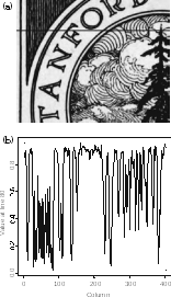 Fig.
5.1 a Original
image and selected line. b
Values
at line 240 original image, selected line, and values at line 80
Fig.
5.1 a Original
image and selected line. b
Values
at line 240 original image, selected line, and values at line 80
bright areas intersected by this strip appear as values close to 1, whereas dark regions correspond to values close to 0.
It is noteworthy how some image features translate into profile variation. See, for instance, the tightly packed vertical dark strips which cross the profile to the left in Fig.5.1a. They appear as a rapidly varying signal in Fig.5.1b. This will be one of the most affected features due to its relatively small size and high contrast. The high values around column 200 correspond to the light region below the “O”, with small variations due to noise.
The following sections will deal with two of the main types of filters that can be defined on the data domain: convolutional and order statistics.