Lektsii (1) / Lecture 11

ICEF, 2012/2013 STATISTICS 1 year LECTURES

We consider new random variable that is some function of an X, i.e. Y = g(X ) . For example X is the net family income and the food expenditure is cX α where α < 1.

Example. Let r.v. X has the following distribution:

and E(X 2 ) = E(Y ) = 0 0.2 +1 0.45 +4 0.35 =1.85 . Alternatively,

E(X 2 ) = (−2)2 0.25 +(−1)2 0.25 +02 0.2 +12 0.2 +22 0.1 =1.85

In order to calculate the expectation E(Y ) one should (according to definition) first construct the distribution (table) of Y:

and then to calculate E(Y ) = ∑yi qi .

i

In fact it may be proved the following statement (that is quite clear intuitively):

E(Y ) = ∑g(xi ) pi .

i

In other words, in order to find the expectation E(Y ) one needs not to construct the distribution of the random variable Y.

Continuous random variables (distributions)

Continuous random variable X has strange and paradoxical property: for any possible value x0 we have Pr(X = x0 ) = 0 . Thus means that we cannot describe the distribution of such random variable via table of distribution similar to discrete r.v.

Alternative description of the distribution of a r.v. X is the probability density function (pdf).

1)f (x) ≥ 0 ;

2)+∞∫ f (x) dx =1 (the square under the curve is equal to 1).

−∞

To define the distribution of a continuous random variable X to define its density function fX (x) .

Definition. If X is a continuous r.v. with the pdf fX (x) then

+∞ +∞

µX = E(X ) = ∫ x fX (x) dx, σX2 =V (X ) = E((X −µX )2 ) = ∫(x −µX )2 fX (x) dx .

−∞ −∞

Standard normal r.v. (distribution)

Definition. Random variable Z is called a standard normal r.v. if

Notation: Z N (0,1) .

It may be calculated that E(Z ) = 0, V (Z ) =1.

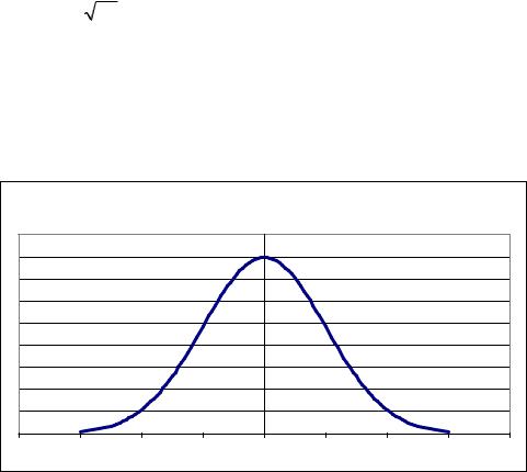
The graph of ϕ(x) is called standard normal curve. It is bell-shaped and symmetric with respect to oy axis.