


264 DESIGN AND ANALYSIS OF PROPOSITIONAL-LOGIC RULE-BASED SYSTEMS
format, with no restrictions on columns or spacing. A comment can be indicated by enclosing it within the character pairs (* *).
Identifiers are used in the program to name variables, constants, and the program name. The rules for forming an identifier are as follows. All alphabetic characters used are lowercase. The first character must be a lowercase alphabetic character: ‘a’. . . ‘z’. All succeeding characters must be alphabetic, numeric, or the underscore character ‘ ’. No special characters or punctuation marks are allowed, and no embedded blanks are allowed. Identifiers may be as long as desired, subject to the restrictions of the system in which EQL is implemented.
10.3.1 The Declaration Section
The declaration of an EQL program consists of three different types of declaration: CONST, VAR, and INPUTVAR. Each type of declaration must appear at most once and in the order indicated above.
10.3.2 The CONST Declaration
The CONST declaration assigns a name to a scalar constant. No predefined constants exist in EQL and thus all constants used in the program must be declared, including the values of the Boolean constants true and false. For example, the following declaration declares four constants.
CONST
false |
= 0 ; |
true |
= 1 ; |
bad |
= 2 ; |
good |
= 3 ; |
10.3.3 The VAR Declaration
All variables used in the program except input variables must be declared in the VAR section. Input variables are those that do not appear on the left-hand-side of any assignment statement. They are used to store the values read from sensors attached to the external environment. For example, the following VAR declaration declares three variables of type BOOLEAN.
VAR
sensor a status, sensor b status, object detected : BOOLEAN ;
10.3.4 The INPUTVAR Declaration
All input variables used in the program must be declared in the INPUTVAR section. For example, the following INPUTVAR declaration declares three input variables of type INTEGER.
PROPOSITIONAL-LOGIC RULE-BASED PROGRAMS: THE EQL LANGUAGE |
265 |
INPUTVAR
sensor a, sensor b, sensor c : INTEGER ;
10.3.5 The Initialization Section INIT and INPUT
All non-input variables are assigned initial or default values in the initialization section INIT before the start of the firing of the rules in the RULES section of the program. For example, the following statements initialize the variables: sensor a status, sensor b status, and object detected.
INIT
sensor a status := good, sensor b status := good, object detected := false
At the beginning of each execution of an EQL program, input values are read into the input variables listed in the READ statement.
INPUT
READ sensor a, sensor b
10.3.6 The RULES Section
The RULES section is composed of a finite set of rules, each of which is of the form:
a1 := b1 ! a2 := b2 ! . . .! am := bm IF enabling condition
A rule has three parts:
VAR = set of variables on left-hand side of the assignment, i.e., the ai s,
VAL = expressions on right-hand side of assignment, i.e., the bi s, and
EC = enabling condition.
A subrule of rule y with m VAR variables is of the form:
c1 := d1 ! c2 := d2 ! . . .! cp := dp IF enabling condition
where each ci is a VAR variable in rule y, di is the expression to be assigned to variable ci in the original rule, and p ≤ m. A single-assignment subrule of rule y is then of the form:
c := d IF enabling condition
where c is a VAR variable in rule y and d is the expression to be assigned to variable c in the original rule.

266 DESIGN AND ANALYSIS OF PROPOSITIONAL-LOGIC RULE-BASED SYSTEMS
An enabling condition is a predicate on the variables in the program. A rule is enabled if its enabling condition becomes true. A rule firing is the execution of the multiple assignment statement. A rule is fireable only when it is enabled and if by firing it will change the value of some variable in VAR. A multiple assignment statement assigns values to one or more variables in parallel. The VAL expressions must be side-effect free. The execution of a multiple assignment statement consists of the evaluation of all the VAL expressions, followed by updating the VAR variables with the values of the corresponding expressions. For ease of discussion, we define three sets of variables for an EQL program:
L = {v | v is a variable appearing in VAR}
R = {v | v is a variable appearing in VAL}
T = {v | v is a variable appearing in EC}
An invocation of an EQL program is a sequence of rule firings (execution of multiple assignment statements whose enabling conditions are true). When two or more rules are enabled, the selection of which rule to fire is nondeterministic or up to the runtime scheduler.
An EQL program is said to have reached a fixed point when none of its rules is fireable. An EQL program is said to always reach a fixed point in bounded time if and only if the number of rule firings needed to take the program from an initial state to a fixed point is always bounded by a fixed upper bound. This bound is imposed by performance constraints. It is possible that a program can reach different fixed points starting from the same initial state, depending on which rules and how the rules are fired. This may suggest that the correctness of the program is violated, whereas for some applications this is acceptable. Our concern in this chapter is, however, on the verification of timing requirements of rule-based programs.
EQL is an equational rule-based language which we have implemented to run under BSD UNIX.1 The current system includes a translator eqtc which translates an EQL program into an equivalent C program for compilation and execution in a UNIX-based machine. The module eqtc and other system modules are implemented in C. An example of an EQL program is shown below.
Example 1. RULES section of a simple object-detection program:
(* 1 *) |
|
object |
detected := true IF sensor |
|
a = 1 AND sensor |
|
a |
|
status = good |
||||
(* 2 *) |
[] |
object |
detected := true IF sensor |
|
b = 1 AND sensor |
b |
status = good |
||||||
(* 3 *) |
[] |
object |
|
|
|
|
|
|
|
|
|
||
detected := false IF sensor |
|
a = 0 AND sensor |
|
a |
|
status = good |
|||||||
(* 4 *) |
[] |
object |
detected := false IF sensor |
|
b = 0 AND sensor |
|
b |
|
status = good |
||||
If sensor a and sensor b read in values 1 and 0, respectively, then the above program will never reach a fixed point since the variable object detected will be set to true and false alternatively by rules 1 and 4. Recall that a rule is enabled if its enabling
1UNIX is a registered trademark of AT&T Bell Laboratories.

PROPOSITIONAL-LOGIC RULE-BASED PROGRAMS: THE EQL LANGUAGE |
267 |
condition is true, and that a rule can fire when it is enabled and if by firing it will change the value of at least one VAR variable. Thus a rule can fire more than once as long as it remains fireable. Rule 1 and rule 4 are said to be not compatible. Similarly, if sensor a and sensor b read in values 0 and 1, respectively, then the above program will never reach a fixed point since the variable object detected will be set to true and false alternatively by rules 2 and 3. Rule 2 and rule 3 are not compatible.
In a real-time system, the goal is to have the decision program converge to a fixed point within a bounded number of rule firings. To ensure that the above decision system will converge to a fixed point given any set of sensor input values, some additional information may be needed to settle the conflicting sensor readings. For example, the following rules may be added to the above program:
5.[] sensor a status := bad IF sensor a = sensor c AND sensor b status = good
6.[] sensor b status := bad IF sensor b = sensor c AND sensor a status = good
where sensor c is an additional input variable. If one of the above two rules is fired, then two of the tests (either tests 1 and 3 or tests 2 and 4) in rules 1–4 will be falsified, thus permanently disabling two of those four rules. The variable object detected will then have a stable value since rules 1 and 4 or rules 2 and 3 can no longer fire alternatively. Since the default scheduler of EQL will eventually fire an enabled rule, all the variables in the above program will converge to stable values after a finite (but unbounded) number of iterations. In section 10.8, we show how this program can be made to converge to stable values in bounded time.
The above example is sufficiently simple that with a little thought one can understand its behavior, and in particular, whether a fixed point can be reached or not. In general, it is non-trivial to determine the behavior of rule-based programs because there is no obvious flow of control. Even small rule-based programs can take quite a bit of work to understand, as the following example illustrates. In a real-time system, the goal is to have the rule-based program converge to a fixed point within a bounded number of rule firings. We would therefore like to determine whether or not the rulebased program will reach a fixed point in a bounded number of rule firings. For a program of this size, the answer is obvious. However, the problem is not trivial for larger programs. In general, the analysis problem to determine whether a rule-based program will reach a fixed point is undecidable if the program variables can have infinite domains, that is, there is no general procedure for answering all instances of the decision problem [Browne, Cheng, and Mok, 1988].
10.3.7 The Output Section
The TRACE statement prints the values of the specified variables following the firing of a rule in each cycle. For example, the following TRACE statement prints the values of the variables sensor a status, sensor b status, and object detected following

268 DESIGN AND ANALYSIS OF PROPOSITIONAL-LOGIC RULE-BASED SYSTEMS
the firing of any rule:
TRACE sensor a status, sensor b status, object detected
The PRINT statement prints the values of the specified variables only after the entire program has reached a fixed point. For example, the following PRINT statement prints the values of the same variables after the program has reached a fixed point.
PRINT sensor a status, sensor b status, object detected
We now show a larger sample EQL program, a distributed program for determining whether an object is detected at each monitor-decide cycle. The system consists of two processes and an external alarm clock which invokes the program by setting the variable wake up to true periodically.
Example 2. Object detection:
(* Example EQL Program *) PROGRAM example2;
CONST
false |
= |
0; |
true |
= |
1; |
a= 0;
b= 1;
VAR
sync_a, sync_b, wake_up,
object_detected : BOOLEAN;
arbiter |
: INTEGER; |
INPUTVAR |
|
sensor_a, |
|
sensor_b |
: INTEGER; |
INIT |
|
sync_a := true, sync_b := true, wake_up := true,
object_detected := false, arbiter := a
INPUT
READ sensor_a, sensor_b
RULES
(* process A *)
object_detected := true ! sync_a := false
IF (sensor_a = 1) AND (arbiter = a) AND (sync_a = true) [] object_detected := false ! sync_a := false
IF (sensor_a = 0) AND (arbiter = a) AND (sync_a = true) [] arbiter := b ! sync_a := true ! wake_up := false
IF (arbiter = a) AND (sync_a = false) AND (wake_up = true)

STATE-SPACE REPRESENTATION |
269 |
(* process B *)
[] object_detected := true ! sync_b := false
IF (sensor_b = 1) AND (arbiter = b) AND (sync_b = true)
AND (wake_up = true)
[] object_detected := false ! sync_b := false
IF (sensor_b = 0) AND (arbiter = b) AND (sync_b = true)
AND (wake_up = true)
[] arbiter := a ! sync_b := true ! wake_up := false
IF (arbiter = b) AND (sync_b = false) AND (wake_up = true)
TRACE object_detected
PRINT sync_a, sync_b, wake_up, object_detected, arbiter, sensor_a, sensor_b END.
In this example, the input variables are sensor a and sensor b, and the program variables are object detected, sync a, sync b, arbiter, and wake up. The three sets of variables L, R, T are:
L = {object detected, sync a, sync b, arbiter, wake up},
R = φ,
T = {sensor a, sensor b, arbiter, sync a, sync b, wake up}.
Each process runs independently of the other. An alarm clock external to the program is used to invoke the processes after some specified period of time. A rule is fired in the same way as in the non-distributed case, namely, the assignment statement is executed when the enabling condition becomes true. In this example, the shared variable arbiter is used as a control/synchronization variable that enforces mutually exclusive access to shared variables, such as object detected, by different processes. The variables sync a and sync b are used as control/synchronization variables within process A and process B, respectively. Note that for each process, at most two rules will be fired before control is transferred to the other process. Initially, process A is given the mutually exclusive access to variables object detected and sync a.
The reader who finds the above example difficult to understand need not be discouraged inasmuch as the point of the example is to impress upon the reader the need for computer-aided tools to design this class of programs. We shall discuss in later sections a set of computer-aided design tools that have been implemented for this purpose. But first, we need to be more precise about the class of systems to which our equational rule-based programs are applied. Then we can formulate the relevant technical questions in terms of a state-space representation.
10.4 STATE-SPACE REPRESENTATION
The state-space graph of an equational rule-based program is a labeled directed graph G = (V, E). V is a set of vertices, each of which is labeled by a tuple: (x1, . . . , xn , s1, . . . , sp), where xi is a value in the domain of the ith input sensor

270 DESIGN AND ANALYSIS OF PROPOSITIONAL-LOGIC RULE-BASED SYSTEMS
variable and s j is a value in the domain of the jth program variable. We say that a rule is enabled at vertex i iff its test is satisfied by the tuple of variable values at vertex i. E is a set of edges, each of which denotes the firing of a rule such that an edge (i, j) connects vertex i to vertex j iff there is a rule R that is enabled at vertex i and firing R will modify the program variables to have the same values as the tuple at vertex j. Whenever no confusion exists, we shall use the terms state and vertex interchangeably. Obviously, if the domains of all the variables in a program are fi- nite, the corresponding state-space graph must be finite. We note that the state-space graph of a program need not be connected.
A path in the state-space graph is a sequence of vertices v1, . . . , vi , vi+1, . . . , such that an edge connects vi to vi+1 for each i. Paths can be finite or infinite. The length of a finite path v1, . . . , vk is k − 1. A simple path is a path in which no vertex appears more than once. A cycle in the state-space graph is a path v1, . . . , vk such that v1 = vk . A path corresponds to the sequence of states generated by a sequence of rule firings of the corresponding program.
A vertex in a state-space graph is said to be a fixed point if it does not have any outedges or if all of its out-edges are self-loops (i.e., cycles of length 1). Obviously, if the execution of a program has reached a fixed point, every rule is either not enabled or its firing will not modify any of the variables.
An invocation of an equational rule-based program can be thought of as tracing a path in the state-space graph. A monitor-decide cycle starts with the update of input sensor variables, and this puts the program in a new state. A number of rule firings will modify the program variables until the program reaches a fixed point. Depending on the starting state, a monitor-decide cycle may take an arbitrarily long time to converge to a fixed point if at all. We say that a state in the state-space graph is stable if all paths starting from it will lead to a fixed point. A state is unstable if none of the paths from it will lead to a fixed point. A state is potentially unstable if there is a path from it that does not lead to a fixed point. By definition, a fixed point is a stable state. It is easy to see that a state s is stable iff any path from s is simple until it ends in a fixed point. A state is potentially unstable iff a cycle is reachable from it or if there is an infinite simple path leading from it.
Figure 10.2 illustrates these concepts. If the current state of the program is A, then the program can reach the fixed point FP2 in four rule firings by taking the path (A, D, F, H, FP2). If the path (A, D, E, . . . , FP1) is taken, the fixed point FP1 will be reached after a finite number of rule firings. State A is stable because all
|
A |
B |
C |
|
|
D |
|
I |
L |
E |
F |
|
J |
M |
|
|
K |
P |
|
|
G |
H |
|
N |
|
FP1 |
FP2 |
FP3 |
|
Figure 10.2 State-space graph of a real-time decision program.
STATE-SPACE REPRESENTATION |
271 |
paths from A will lead to a fixed point. If the current state of the program is B, the program will iterate forever without reaching a fixed point. All the states {B, I, J, K } in the cycle (B, I, J, K , B) are unstable. Note that no out-edge is present from any of the states in this cycle. Once the program enters one of these states, it will iterate forever. If the current state of the program is C, the program may enter and stay in a cycle if the path (C, L, J, . . .) is followed. If the path (C, L, M, . . .) is taken, the cycle (M, P, N, M) may be encountered. The program may eventually reach the fixed point FP3 if at some time the scheduler fires the rule corresponding to the edge from P to FP3 when the program is in state P. To ensure this, however, the scheduler must observe a strong fairness criterion: if a rule is enabled infinitely often, it must be fired eventually. In this case, paths from state C to FP3 are finite but their lengths are unbounded. C is a potentially unstable state.
In designing real-time decision systems, we should never allow an equational rule-based program to be invoked from an unstable state. Potentially unstable states can be allowed only if an appropriate scheduler is used to always select a sufficiently short path to a fixed point whenever the program is invoked from such a state. We say that a fixed point is an end-point of a state s if that fixed point is reachable from s. It should be noted that not every tuple that is some combination of sensor input and program variable values can be a state from which a program may be invoked. After a program reaches a fixed point, it will remain there until the sensor input variables are updated, and the program will then be invoked again in this new state. The states in which a program is invoked are called launch states. Formally, we define a launch state2 as follows:
1.The initial state of a program is a launch state.
2.A tuple obtained from an end point (which is a tuple of input and program variables) of a launch state by replacing the input variable components with any combination of input variable values is a launch state.
3.A state is a launch state iff it can be derived from rules (1) and (2).
In this chapter, the timing constraint of interest is a deadline that must be met by every monitor-decide cycle of an equational rule-based program. In terms of the state-space representation, the timing constraint imposes an upper bound on the length of paths from a launch state to a fixed point. Integrity constraints are assertions that must hold at the end points of launch states. Given a program that meets the integrity constraints but violates the timing constraint, the synthesis problem is to transform this program into one that also meets the timing constraint. This can be done by program transformation techniques and/or by customizing the scheduler to
2The above definition of a launch state is conservative in the sense that not all combinations of input variables need to be considered in the construction of launch states because future sensor readings are restricted by the environmental constraints. However, since environmental constraints are necessarily approximations of the external world, it seems prudent not to include them in the definition of a launch state. We emphasize that it is possible to take advantage of environmental constraints in cutting down the number of launch states for analysis purposes.
272 DESIGN AND ANALYSIS OF PROPOSITIONAL-LOGIC RULE-BASED SYSTEMS
fire the rules selectively so that an invocation always fires the rules corresponding to the shortest path from the launch state to an end point.
In the next section, we shall describe some of the tools that we have implemented to mechanize the analysis problem, that is, to determine if the upper bound on the monitor-decide cycle can indeed be met in the worst case. Some of the theoretical issues related to the analysis and synthesis problems will be discussed in sections 10.6 and 10.8.
10.5 COMPUTER-AIDED DESIGN TOOLS
The complexity and size of real-time decision systems often necessitate the use of computer-aided design tools. This chapter reports on a suite of analysis tools that have been implemented to ensure that equational rule-based programs written in the language EQL can indeed meet their specified timing and integrity constraints. In particular, the tools are used to perform a pre-run-time analysis on an EQL program to verify that the variables in the program will always converge to stable values in bounded time at each invocation.
As in the design of most complex software systems, we envision the development of real-time rule-based systems to be an iterative process. Our goal is to speed up this iterative process by automating it as much as possible. Figure 10.3 shows the interaction of a designer with the tools. In each design cycle, the equational rulebased program is analyzed by the analysis tools for compliance with the timing and integrity constraints. Violations are passed to the designer who can then modify the program with the help of the synthesis tools until the program meets all the constraints. It should be emphasized, however, that the purpose of the design tools is not to encourage people to write sloppy programs and rely on the tools to fix them. Design tools are particularly necessary for rule-based programs because the addition and/or deletion of just one rule may drastically change the behavior of a program,
|
Analysis Tool |
|
Real Time |
Possible Hazards |
|
and |
||
|
||
Decision Program |
Timing Violations |
|
User Interaction |
|
|
|
Synthesis |
|
|
Transformation |
|
|
Tools |
Figure 10.3 Development of real-time decision systems.
COMPUTER-AIDED DESIGN TOOLS |
273 |
and it is essential to guard against unintended interference in the work of individual members of a design team.
In this chapter, our main focus is on a suite of analysis tools that have been implemented for the equational rule-based language EQL. For efficient execution, a translator of EQL programs into C code exists. We selected C as the target language since it is widely available and has efficient compilers. Since EQL has nondeterministic constructs, our translator generates the appropriate C code to simulate nondeterminism and parallelism on a sequential machine.
Our software tools provide:
1.a translator for transforming an EQL program into its corresponding statespace graph as described in the previous section. The state-space graph serves as an intermediate form of the program under development and is used for mechanical analysis and synthesis.
2.a temporal-logic verifier for checking integrity assertions about EQL programs. (In the current implementation, these assertions can be expressed in the temporal logic called computation tree logic [Clarke, Emerson, and Sistla, 1986] described in chapter 4.) Specifically, the verifier determines, given any launch state, whether some fixed points are always reachable in a finite number of iterations and whether the reachable fixed points are safe, that is, satisfy the specified integrity constraints. If the given EQL program cannot reach a fixed point from a particular launch state, the temporal-logic verifier will warn the designer of the existence of a cycle that does not have a path exiting from it.
3.a timing analyzer for determining the maximum number of iterations to reach a safe fixed point, and the sequence of states traversed (along with the sequence of rules fired) from the launch state to the fixed point. This helps the designer pinpoint the sets of rules that may constitute a performance bottleneck so that optimization efforts can be concentrated on them. The timing analyzer can also be used to investigate the performance of customized schedulers that are used to deterministically select a rule to fire when two or more rules are enabled.
A suite of practical prototyping tools has been implemented on a Sun Microsystems3 workstation running under UNIX BSD 4.2 to perform timing and safety analysis of real-time equational rule-based programs. Although these are the first versions of the analysis tools, they are nonetheless sufficiently practical for analyzing realistic real-time decision systems. To demontrate their usefulness, we have used these tools to verify that a subset of the Cryogenic Hydrogen Pressure Malfunction Procedure of the Space Shuttle Vehicle Pressure Control System will reach a safe fixed point in a finite number of iterations from any launch state.
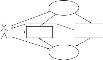
Figure 10.4 illustrates the dependency among the modules in our tool system. The names of the modules and descriptions of their functions follow:
1.eqtc – EQL to C translator
2.ptf – EQL to finite state-space graph translator for a launch state
3SUN is a registered trademark of SUN Microsystems Inc.

274 DESIGN AND ANALYSIS OF PROPOSITIONAL-LOGIC RULE-BASED SYSTEMS
equational |
customized |
|
rule-based program |
scheduler specification |
|
|
|
|
|
|
|
|
|
|
|
|
|
eqtc |
|
ptf |
|
|||
|
|
|
|
|
|
|
|
|
|
|
|
||
C program |
finite state-space graph |
|||||
CTL temporal logic formula |
||||||
|
|
|||||
|
|
|
|
|
|
|
|
|
|
|
|
|
|
|
|
|
|
|
|
|
|
|
|
|
|
|
|
C Compiler |
|
mcf |
|
|
fptime |
|
|||
|
|
|
|
|
|
|
|
|
|
|
|
|
|
|
|
|
|
|
|
executable |
indicates whether |
maximum number of |
|||||||
C object code |
|
a fixed point is |
iterations to reach |
||||||
|
|
|
always reached |
a fixed point and the |
|||||
|
|
|
|
|
|
sequence of rules fired |
|||
Figure 10.4 Computer-aided design tools for real-time decision systems.
3.ptaf – EQL to finite state-space graphs translator for all launch states
4.mcf – CTL model checker (extended to cover fairness)
5.fptime – Timing analyzer on state-space graphs
The module eqtc translates a program written in the equational rule-based language EQL into a C program suitable for compilation using the cc compiler under UNIX, as described earlier. EQL is a Unity-based language with nondeterministically scheduled rules and parallel assignment statements.
The module ptf translates an EQL program with finite domains (all variables have finite ranges) into a finite state-space graph that contains all the states reachable from the launch state corresponding to the initial values of the variables given in the program. It also generates the appropriate temporal-logic formula for checking whether the program will reach a fixed point. ptf produces a file named mc.in which will be read by the fairness-extended model checker mcf and the timing analyzer module fptime. The file mc.in contains the internal representation of the state-space graph of the corresponding EQL program.
The module ptaf is similar to ptf, but it automatically generates the complete state-space graph (i.e., it generates all the states reachable from every launch state). ptaf invokes the model checker and the timing analyzer to determine whether the program will reach a fixed point in a finite number of iterations, starting from any