

TsOS / DSP_guide_Smith / Ch32
.pdfChapter 32The Laplace Transform
|
R |
|
|
|
|
|
C |
|||
|
|
|
|
|
|
|||||
|
|
|
|
|||||||
Vin |
R |
|||||||||
|
|
|
|
|
|
|
A |
|
|
|
|
|
|
|
|
|
|
|
|
|
|
|
|
C |
|
|
|
|
|
Vout |
||
|
|
|
|
|
|
|
|
|||
|
|
|
|
|
|
|
||||
|
|
|
|
|
|
|
|
|
|
|
|
|
|
|
|
|
|
|
|
|
|
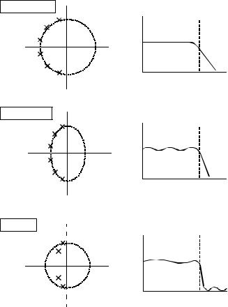
FIGURE 32-9
Sallen-Key characteristics. This circuit produces two poles on a circle of radius 1/RC. As the gain of the amplifier is increased, the poles move from the real axis, as in (a), toward the imaginary axis, as in (d).
jT
a. A = 1.0
F |
|
|||
|
|
|
|
|
2 poles |
|
|||
|
|
|
|
jT |
b. A = 1.586 |
|
|||
|
|
|||
F |
|
|||
|
|
|
|
|
jT
c. A = 2.5
F
jT
d. A = 3.0
F
601
T0
Amplitude
Frequency
T0
Amplitude
Frequency
T0
Amplitude
Frequency
T0
Amplitude
Frequency
As the amplification is increased, the poles move along the circle, with a corresponding change in the frequency response. As shown in (b), an amplification of 1.586 places the poles at 45 degree angles, resulting in the frequency response having a sharper transition. Increasing the amplification further moves the poles even closer to the imaginary axis, resulting in the frequency response showing a peaked curve. This condition is illustrated in (c), where the amplification is set at 2.5. The amplitude of the peak continues to grow as the amplification is increased, until a gain of 3 is reached. As shown in (d), this is a special case that places the poles directly on the imaginary axis. The corresponding frequency response now has an infinity large value at the peak. In practical terms, this means the circuit has turned into an oscillator. Increasing the gain further pushes the poles deeper into the right half of the s- plane. As mentioned before, this correspond to the system being unstable (spontaneous oscillation).
Using the Sallen-Key circuit as a building block, a wide variety of filter types can be constructed. For example, a low-pass Butterworth filter is designed by placing a selected number of poles evenly around the left-half of the circle, as shown in Fig. 32-10. Each two poles in this configuration requires one

602 |
The Scientist and Engineer's Guide to Digital Signal Processing |
Sallen-Key stage. As described in Chapter 3, the Butterworth filter is maximally flat, that is, it has the sharpest transition between the passband and stopband without peaking in the frequency response. The more poles used, the faster the transition. Since all the poles in the Butterworth filter lie on the same circle, all the cascaded stages use the same values for R and C. The only thing different between the stages is the amplification. Why does this circular pattern of poles provide the optimally flat response? Don't look for an obvious or intuitive answer to this question; it just falls out of the mathematics.
Figure 32-11 shows how the pole positions of the Butterworth filter can be modified to produce the Chebyshev filter. As discussed in Chapter 3, the Chebyshev filter achieves a sharper transition than the Butterworth at the expense of ripple being allowed into the passband. In the s-domain, this corresponds to the circle of poles being flattened into an ellipse. The more flattened the ellipse, the more ripple in the passband, and the sharper the transition. When formed from a cascade of Sallen-Key stages, this requires different values of resistors and capacitors in each stage.
Figure 32-11 also shows the next level of sophistication in filter design strategy: the elliptic filter. The elliptic filter achieves the sharpest possible transition by allowing ripple in both the passband and the stopband. In the s- domain, this corresponds to placing zeros directly on the real axis, with the first one near the cutoff frequency. Elliptic filters come in several varieties and are significantly more difficult to design than Butterworth and Chebyshev configurations. This is because the poles and zeros of the elliptic filter do not lie in a simple geometric pattern, but in a mathematical arrangement involving elliptic functions and integrals (hence the name).
1 pole |
jT |
2 pole |
jT |
F |
|
F |
|
FIGURE 32-10
The Butterworth s-plane. The low-pass Butterworth filter is created by placing poles equally around the left-half of a circle. The more poles used in the filter, the faster the roll-off.
3 pole |
|
|
jT |
|
6 pole |
|
|
jT |
||
|
|
|||||||||
F |
|
|
|
F |
|
|
||||
|
|
|
|
|
|
|
|
|
|
|
|
|
|
|
|
|
|
|
|
|
|
Chapter 32The Laplace Transform
FIGURE 32-11
Classic pole-zero patterns. These are the three classic pole-zero patterns in filter design. Butterworth filters have poles equally spaced around a circle, resulting in a maximally flat response. Chebyshev filters have poles placed on an ellipse, providing a sharper transition, but at the cost of ripple in the passband. Elliptic filters add zeros to the stopband. This results in a faster transition, but with ripple in the passband and stopband.
Butterworth jT
F
Chebyshev jT
F
Elliptic |
o |
jT |
|
|
|
|
o |
|
F |
|
|
|
o |
|
|
o |
|
603
 T0
T0
Amplitude
Frequency
 T0
T0
Amplitude
Frequency
T0
Amplitude
Frequency
Since each biquad produces two poles, even order filters (2 pole, 4 pole, 6 pole, etc.) can be constructed by cascading biquad stages. However, odd order filters (1 pole, 3 pole, 5 pole, etc.) require something that the biquad cannot provide: a single pole on the imaginary axis. This turns out to be nothing more than a simple RC circuit added to the cascade. For example, a 9 pole filter can be constructed from 5 stages: 4 Sallen-Key biquads, plus one stage consisting of a single capacitor and resistor.
These classic pole-zero patterns are for low-pass filters; however, they can be modified for other frequency responses. This is done by designing a low-pass filter, and then performing a mathematical transformation in the s-domain. We start by calculating the low-pass filter pole locations, and then writing the transfer function, H (s), in the form of Eq. 32-3. The transfer function of the corresponding high-pass filter is found by replacing each "s" with "1/s", and then rearranging the expression to again be in the pole-zero form of Eq. 32-3. This defines new pole and zero locations that implement the high-pass filter. More complicated s-domain transforms can create band-pass and band-reject filters from an initial low-pass design. This type of mathematical manipulation in the s-domain is the central theme of filter design, and entire books are
604 |
The Scientist and Engineer's Guide to Digital Signal Processing |
devoted to the subject. Analog filter design is 90% mathematics, and only 10% electronics.
Fortunately, the design of high-pass filters using Sallen-Key stages doesn't require this mathematical manipulation. The "1/s" for "s" replacement in the s-domain corresponds to swapping the resistors and capacitors in the circuit. In the s-plane, this swap places the poles at a new position, and adds two zeros directly at the origin. This results in the frequency response having a value of zero at DC (zero frequency), just as you would expect for a high-pass filter. This brings the Sallen-Key circuit to its full potential: the implementation of two poles and two zeros.