

Usher Political Economy (Blackwell, 2003)
.pdf292 |
V O T I N G |
of 11 students who decide collectively how many spears to buy. Spears cost $550 each, and there is a firm agreement among the students in the class that (1) total expenditure on spears is to be borne equally by every student (so that, if the class decides to buy 5 spears altogether, the cost to each student is $250 [(5 × 550) ÷ 11] and that (2) the number of spears purchased is to be determined by majority rule voting. Each student’s preferred number of spears for the class is a trade-off in his assessment of the cost of spears – the loss of other goods from his share of the expenditure on spears – and the benefit of fighting effectively. Students can then be lined up – “doves” to the left and “hawks” to the right – in accordance with the number of spears they want the class to buy. Suppose it just so happens that the first and least-hawkish student wants the class to buy 1 spear, the second wants the class to buy 2 spears, the third to buy 3, and so on until the eleventh and most hawkish student wants the class to buy 11 spears. Suppose also that, in a choice between two numbers of spears, a person always prefers the number of spears that is closest to his first preference.
The outcome of the vote is now determinate. As long as each student votes his true preference in any pair-wise vote, the class votes to buy 6 spears, for the number 6 wins against any other number. To see why this is so, suppose person six proposes 6 spears and person nine proposes 9 spears. In this contest, everybody who wants 9 or more spears votes for 9 against 6; everybody who wants 6 or less spears votes for 6 over 9. Person seven votes for 6 spears, and person eight votes for 9 spears. Six spears wins because the six people who want 6 spears or less (and who therefore vote for 6 six spears over 9 spears) constitute a majority of the eleven voters. An analogous argument establishes that 6 spears also wins in a pair-wise vote against any smaller number because more than half the voters want 6 or more spears and are therefore prepared to vote for 6 over any smaller number. Six spears wins because it is the first preference of the median voter, the voter in the middle, when all voters are lined up according to their first preferences on some common scale.
This example immediately generalizes to all public goods, defined in chapter 5 as yielding benefits that accrue to everybody simultaneously, as long as each person’s share of the total cost is set in accordance with an agreed-upon rule of taxation. Total expenditure on roads, police, public education, public transport or public health usually conform, more or less, to this pattern. People differ in their preferences for public goods, but an electoral equilibrium emerges regardless.
The marked contrast between the determinacy in voting about the number of spears and the indeterminacy in voting about ham, cheese, and tuna sandwiches calls for a general explanation of why the examples differ and of the relevance of the examples to the stability of voting in actual democratic societies. What is it about the one example that avoids the pitfalls of the other? The main difference between the spears example and the ham, cheese, and tuna example lies in the possibility of ordering options on an electorally meaningful scale. In the spears example, people need not agree about which option is best, but their preferences for spears can be ordered in a way that voters’ preferences for ham, tuna, and cheese sandwiches cannot. To see what this means, simplify the spears example by reducing the size of the class from eleven students to three students called A, B, and C, and consider only three military options – large expenditure, medium expenditure, and small expenditure. Person A

V O T I N G |
293 |
Table 9.3 Two constellations of preferences for military expenditure
There exists an equilibrium of voting
|
First |
Second |
Last |
People |
preference |
preference |
preference |
|
|
|
|
A |
Large |
Medium |
Small |
B |
Medium |
Small |
Large |
C |
Small |
Medium |
Large |
|
|
|
|
There exists no equilibrium of voting
|
First |
Second |
Last |
People |
preference |
preference |
preference |
|
|
|
|
A |
Large |
Medium |
Small |
B |
Medium |
Small |
Large |
C |
Small |
Large |
Medium |
|
|
|
|
is a hawk whose preferences are for large, medium, and small military expenditure in that order. Person C is a dove whose preferences are just the opposite, for small, medium, and large military expenditure in that order. Person B is a slightly dovish moderate whose preferences are for medium, small and large military expenditure in that order. Their preferences are set out in the left-hand side of table 9.3.
The outcome of the vote is immediately obvious from inspection of table 9.3. Person B’s preference prevails. Medium expenditure wins in a pair-wise vote with either of the other two options. Person B combines with person A to vote for medium expenditure against small expenditure, and person B combines with person C to vote for medium expenditure against large expenditure. With this constellation of preferences, the three-person example is exactly analogous to the eleven-person example we examined before.
The right-hand side of table 9.3 is almost the same. Preferences of persons A and B are exactly the same. The first preference of person C is the same as well, but his second and third preferences are reversed. Now, though person C’s first preference is for small expenditure, he is nevertheless assumed to prefer large to medium expenditure. One might imagine that person C, and person C alone, is of the opinion that the extra expenditure in passing from small to medium is useless because the extra spears would be insufficient to attain victory over one’s enemies, but that large expenditure would be effective though still not worth the price. Regardless, the small change in the preferences of person C upsets the voting equilibrium completely. Formerly, medium expenditure won in a pair-wise vote with either large or small expenditure because medium expenditure was always the first preference of one voter and the second preference of the other two. Now, that is no longer so, though neither of the other two options can displace medium expenditure altogether. All three options are on equal footing, and none can win in both pair-wise votes with the other two. There is, in fact, an exact correspondence between the right-hand side of table 9.3 and the ham, tuna, and cheese example in table 9.2 above: large replacing ham, medium replacing tuna, and small replacing cheese. The ordering of options on a common scale that created an electoral equilibrium in the original spear example is missing in the example illustrated on the left-hand side of table 9.3. A natural ordering is sometimes present in actual voting, and sometimes not.
A more precise specification of the conditions for an electoral equilibrium can be obtained from a generalization of our example. Consider once again the guns and butter economy discussed in chapter 5. Suppose everybody works the same number of hours per day, but people differ in their tastes and in their productivities of labor.
294 |
V O T I N G |
Think of each person i as producing yiG units of output in that time, where a unit of output consists of either one pound of butter or one gun. The output, yiG, of person i is his gross, pre-tax income. As there is no investment in this guns and butter economy, a person’s net, post-tax income can only be spent on butter.1 The net post-tax income, yiN, of person i and his consumption of butter are one and the same. Each person i has a unique utility function ui(yiN, G) where yiN is his consumption of butter and G is society’s total production of guns. From a person’s utility function, there may be constructed a set of indifference curves, with the same general shape as the indifference curves in figure 5.1. Suppose, finally, that there is an inflexible rule in this society that all taxation is directly proportional to income, so that a person’s consumption of butter is equal to
yiN = yiG(1 − t) |
(5) |
where t is society’s chosen rate of taxation. Total tax revenue is tyN where t is the tax rate, y is average pre-tax income in the economy as a whole, and N is total population. The government uses the revenue from taxation to employ people to produce guns. Since, by assumption, one unit of labor is required to produce one gun, the total supply of guns, G, is just equal to total revenue. The government’s budget constraint is
G = tyN |
(6) |
Utility functions can now be reconstructed as dependent on the total output of guns.
ui(yiN, G) = ui(yiG(1 − t), G) = ui(yiG(1 − G/yN), G) = ui(G) |
(7) |
The utility, welfare, or well-being of person i depends in the first instance on both the quantity of butter he consumes and the number of guns his government acquires for the defense of the realm. His utility can nevertheless be expressed as dependent on the number of guns alone because average income, population, and his own pre-tax income are what they are regardless of society’s choice of the number of guns, but his consumption of butter (his post-tax income) is determined by the number of guns when the tax rate is just sufficient to finance the guns that the government chooses to buy. Utility depends upon G alone not because the other terms have suddenly become irrelevant, but because the other terms are either invariant or determined once G is chosen. The terms yiG (gross income of person i), y (average income), and N (population) have been assumed invariant. The tax rate, t, depends on the choice of G.
It is critical in what follows that every person’s utility function, ui(G), be hiveshaped as illustrated in figure 9.3 rather than wavy, in other words, that the utility function be single peaked. Every person i must have a preferred value of G, called Gi in figure 9.3. Extra guns would not be worth the extra tax he would have to pay to finance them. Fewer guns would reduce his security by more than the value of the corresponding reduction in taxation. To assume preferences are single-peaked is to suppose that every person’s utility diminishes steadily the farther away society’s choice of G happens to be from his first preference Gi. To use a different example, a person whose political preference is in the center of the political spectrum prefers policies on
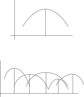
Utility of person i (ui)
V O T I N G |
295 |
ui(G)
Gi
Output of guns (G)
Figure 9.3 Person i’s preference for guns.
Utility
u4
u1 |
u2 |
|
|
u3 |
|
|
u5 |
||
|
|
|
|
|
G4 |
G1 |
G2 |
G5 |
G3 |
|
|
Output of guns |
|
|
Figure 9.4 Identifying the median voter.
the moderate right to policies on the extreme right. All preferences on the left-hand side of table 9.3 and the preferences of persons A and B on the right-hand side are single peaked. The preference of person C on the right-hand side of table 9.3 is not. While by no means impossible, person C’s preference ordering is unusual and will be ignored in the analysis to follow. The assumption that all preferences are single peaked is important because, without it, the electoral equilibrium may fail to appear.
People need not agree upon the best number of guns for their government to procure, but disagreement can be resolved by voting. Imagine a society of five people with different utility functions, ui(xi, G) for i = 1 to 5, and different gross incomes, yiG. A distinct hive-shaped utility function like that in figure 9.3 can be constructed for each person. Since incomes and utility functions differ among the five people, the functions ui(G) would differ as well. Each person i has a different preferred quantity of guns, Gi, corresponding to the top of his utility function. Suppose preferences turn out to be as shown in figure 9.4. Person 3 wants the most guns, person 5 next, person 2 next, person 1 next, and person 4 least.
The outcome of voting about the number of guns in this five-person society is very different from the outcome of voting in the examples of the paradox of voting and
296 |
V O T I N G |
the exploitation problem as discussed above. There an electoral equilibrium eluded us. Here a unique equilibrium emerges. An electoral equilibrium, if there is one, is a number of guns chosen over any other number of guns in a pair-wise vote. It is immediately evident there is an electoral equilibrium number of guns, and that it is G2, the first preference of person 2. The reason is exactly the same as in the spears example. In fact, the guns and butter example is the spears example with each person’s preference about the number of spears grounded in the circumstances of the economy and his utility function for spears and for whatever else money can buy. When the five voters’ preferred numbers of guns are lined up from smallest to largest as shown on the horizontal axis of figure 9.4, the first preference of person 2, G2, is in the middle of the line with as many first preferences to the left as to the right. Person 2 is said to be the median voter. A majority of voters can always be found to vote for G2 against any other option. G2 guns wins in any pair-wise vote against any larger number of guns because everybody who would prefer fewer than G2 guns votes together with person 2 for G2. Similarly, G2 wins in any pair-wise vote against any smaller number of guns because everybody who would prefer more guns than G2 votes together with person 2 for G2. Generalizing from this example, it may be said that “the first preference of the median voter is an electoral equilibrium when all preferences are single peaked.” [A minor adjustment to this statement is required if the number of voters is even rather than odd.] Many issues are single-peaked.
A critical assumption in the spear example was that, however many spears are purchased, the total expenditure on spears is allocated equally among all voters. The corresponding assumption in the guns and butter example was that, high or low, the tax rate is the same for everybody. In both examples, the tax convention was the outcome of a prior agreement that everybody continues to respect. Either convention (and a number of other conventions besides) would do, but one convention must somehow be chosen to keep the exploitation problem at bay, for the choice by voting of each person’s tax bill, one by one, is analogous to the allocation of $700,000 by voting, with the unimportant exception that people receive in one case and the government takes in the other. Voting on tax shares would automatically create a classic exploitation problem, as described above in the discussion of the diseases of democracy. If tax shares were determined by majority rule voting, a majority coalition might well form – based on gender or language or religion or race or anything else – to shift the entire burden of the cost of spears onto the excluded minority. That outcome can only be blocked by a prior agreement restricting the scope of voting so that the problem does not arise.
A unique electoral equilibrium may also emerge in voting about the redistribution of income. Voting about the redistribution of income may be more like voting about the number of spears than like voting about the allocation of a fixed sum of money, but, to avoid the pitfalls of faction, the vote must be about one number representing the degree of redistribution and governing the entire pattern of redistribution in the economy as a whole. Consider once again the negative income tax which was the vehicle in an earlier example for the expropriation of the rich by the poor. Continue to suppose that the income of the median voter (the voter half way along the scale from the very poorest person to the very richest person) is less than the average income (total income divided by the number of people), as is the case in actual societies where
V O T I N G |
297 |
the income distribution is always skewed. In the earlier example, the median voter favored 100 percent redistribution, destroying all incentive to work and save.
There was something fishy about that example. Surely, if 100 percent redistribution is destructive, it would be in everyone’s interest to desist from 100 percent redistribution. Nobody would vote for complete redistribution of income for fear of killing the goose that lays the golden eggs. The weak point in the argument is the assumption that income per head remains invariant regardless of whether or to what extent the income is shared through the intermediary of taxation. The argument breaks down when the pie contracts as you share it or when redistribution of income diminishes total income by weakening the tax payer’s incentive to work and to save and by diverting the energies of the taxpayer from production to tax evasion. With complete redistribution of income, there would soon be little income left to redistribute, and even the very poor would become worse off than if there had been no redistribution at all. Another way of expressing this concern is to say that taxation is costly, not just in the sense that the tax collector has to be paid, but in the more important sense that taxation provides tax payers with incentives to take actions yielding small benefits to themselves while generating large harms to others. The “proof ” that the poorer half of the population would vote for 100 percent redistribution required that taxation be costless. That is never so, and the proposition disintegrates when the costliness of taxation is taken into account.
The disintegration is not complete, and a residue of the proposition remains even when the tax-induced contraction of the national income is recognized. Consider a community of three people who all work 12 hours a day, who differ in their earnings per hour, who redistribute income through a negative income tax and who choose the tax rate by majority rule voting. The first person earns $20 per hour, the second earns $10 per hour, and the third earns $6 per hour, and their daily incomes are $240, $120, and $72 respectively. Their average income is $144 a day, and their median income is $120 a day. The community votes for a tax rate, t, to finance a lump sum transfer, T, for everybody. There is no other government expenditure. A tax rate of 0 percent means that there is no redistribution. A tax rate of 100 percent would ensure that everybody’s post-tax, post-transfer income is the same. As long as the average income remains invariant no matter what tax rate is chosen, the community votes two-to-one for a negative income tax at a rate of 100 percent because the low-wage person earning $72 per day and the middle-wage person earning $120 per day are both better off than they would be at any other tax rate. The high-wage person is correspondingly worse off, but, as long as the mean income is greater than the median, he is consistently outvoted. So far, the pessimistic conclusion of our earlier example is borne out.
The key assumption generating this inference is that everybody’s pre-tax income is independent of the tax rate. The assumption is that the declared taxable incomes of $24, $120, and $72 per day are what they are regardless of whether and at what rate they are taxed. There are several reasons why this might not be so. As the tax rate increases, tax payers might switch from taxed work for pay to untaxed leisure or do-it- yourself activities. They might resort to untaxed barter or might find ways of concealing ever-larger shares of their incomes from the tax collector. Tax payers’ allocation of time would be irrelevant if taxation could be levied as a fixed amount per head, or made dependent upon the taxpayer’s ability as indicated by his wage per hour, or set in

298 |
V O T I N G |
Table 9.4 The productivity of do-it-yourself activities
[A person can devote at most 1 hour to each activity. Time not devoted to do-it-yourself activities is devoted to work for pay.]
|
Rank of |
Value of output |
Activity |
activity |
per hour ($) |
|
|
|
Cooking |
I |
18 |
House cleaning |
II |
16 |
Flower gardening |
III |
14 |
Vegetable gardening |
IV |
12 |
Washing clothes |
V |
10 |
Snow removal |
VI |
8 |
Window cleaning |
VII |
6 |
Home repair |
VIII |
5 |
Mending clothes |
IX |
4 |
Wood chopping |
X |
3 |
Plumbing |
XI |
2 |
Electrical repair |
XII |
1 |
|
|
|
accordance with any attribute of the taxpayer that is unaffected by the tax rate. A head tax is technically feasible, but obviously unsuitable as a source of income for redistribution. An ability tax is infeasible because the tax collector has no accurate measure of people’s abilities. Nor can the government observe and evaluate people’s do-it-yourself activities. In practice, there is really no alternative to an income tax exempting leisure, barter, and do-it-yourself activities.
To explain why a majority of self-interested voters prefer redistribution well short of 100 percent, it is sufficient to consider the switch from taxed work for pay to untaxed do-it-yourself activities. Continue to assume that each person works for exactly 12 hours a day, but suppose the available 12 hours can be allocated between work for pay which is taxed and do-it-yourself activities which are not. Assume also that, though they earn different wages per hour, the three people have the same options for do- it-yourself activities. Each person may devote up to one hour to each of the twelve do-it-yourself activities in table 9.4. The do-it-yourself activities are listed in the lefthand column and numbered with Roman numerals in the middle column according to their productivities. The right-hand column shows the productivity of each do-it- yourself activity, measured as the number of dollars it would cost to purchase an hour’s worth of that activity in the market. Thus, the number 12 for vegetable gardening means that it would cost $12 to buy the equivalent of what one grows for oneself in one hour of vegetable gardening.
Every person requires all of the services listed in table 9.4, but each person produces for himself only those services that he cannot acquire from the market at an expenditure of less than an hour of work. If my after-tax income from paid work is $15 per hour, I do an hour of cooking and an hour of house-cleaning but no other do-it-yourself activities, leaving 10 hours for paid work. If my after-tax income from work is $13 per hour, I do an hour of flower gardening as well, and an hour less paid work. If
V O T I N G |
299 |
my after-tax wage exceeds $18, I engage in no do-it-yourself activities at all. If my after-tax wage is less than $1, I engage in 12 hours of do-it-yourself activities and do no paid work. Every person has a critical do-it-yourself activity; he engages in that activity and all lower-numbered activities, but no higher-numbered activities.
For each of the three people – whose earnings are $20, $10, and $6 per hour – and for every tax rate from 0 to 100 percent, one can tell which do-it-yourself activities are advantageous for that person, and, consequently, what his income from do-it-yourself activities, his income from paid work, his tax paid, his total after-tax income, and his total production will be. This information, which is easily computed, is presented in the three parts of table 9.5. The story for the high-wage person is told in table 9.5a. The story for the middle-wage person is told in table 9.5b. The story for the low-wage person is told in table 9.5c. In all three tables, the gradual rise in the tax rate from 0 to 100 percent has two principal effects: (1) The amount of tax paid begins at 0 when the tax rate is 0 percent, gradually increases together with the tax rate, reaches a peak at a tax rate that is well short of 100 percent, and then declines, falling to 0 again when the tax rate reaches 100 percent. (2) The value of total production – inclusive of the output of paid work and the value of do-it-yourself activities – falls steadily as the tax rate rises from 0 to 100 percent.
Though the tax rate could be anything from 0 to 100 percent, it is sufficient for our purposes to tabulate the effects of taxation on each tax payer for eleven rates, including a rate of 0 percent and a rate of 1 percent, which is too low to affect anybody’s choice of do-it-yourself activities. For each tax rate, the after-tax earning per hour of work is shown in column (2) and the choice of do-it-yourself activities is listed in column (3). For example, at a tax rate of 41 percent, a person with a wage of $20 per hour has an after-tax income of $11.80 per hour [(1 − 0.41) × 20 = 11.8]. From table 9.4 above, one can see that a person can earn more than $11.80 at the first four do-it-yourself activities – cooking, cleaning, flower gardening, and vegetable gardening – but at no others. He is shown in figure 9.5a as engaging in those activities, yielding him benefits worth $60[18 + 16 + 14 + 12]. As he has 12 hours of time in total, he devotes only 8 hours to paid work, earning $160 per day as shown in column (5). The high-wage person pays $65.60 tax as shown in column (6). As shown in the final column, his total production, from paid work and do-it-yourself activities, falls steadily from a maximum of $240 when the tax rate is 0 percent to a minimum of $99 when the tax rate reaches 100 percent, the $99 being the sum of the returns from all twelve do-it-yourself activities.
The cause of the fall in production is the tax-induced substitution of less productive but untaxed activities for more productive but taxed activities. At paid work, a highwage person who can earn $20 per hour before tax must be producing goods worth $20 per hour. When the tax rate is 41 percent, his net, after-tax earnings are only $11.80 per hour. At that rate of remuneration, it becomes advantageous for him to divert four hours from paid work to the four most productive do-it-yourself activities: cooking, house cleaning, flower gardening and vegetable gardening. For the highwage person himself, the diversion is advantageous, the acquisition of $60 worth of output from do-it-yourself in exchange for $47.20 [11.80 × 4] of income from paid work. For society as a whole, the diversion is harmful, the acquisition of $60 of

300 |
|
|
|
V O T I N G |
|
|
|
|
|
Table 9.5a The high-wage tax payer’s response to taxation |
|
||||||
|
[This person’s wage is $20 per hour.] |
|
|
|
|
|||
|
|
|
|
|
|
|
|
|
|
|
|
|
(4) |
(5) |
|
(7) |
|
|
|
(2) |
|
Income |
Income |
|
Total |
(8) |
(1) |
After-tax |
(3) |
from do-it- |
from |
(6) |
after-tax |
Total |
|
|
Tax |
earnings |
Do-it- |
yourself |
paid |
Tax |
income |
production |
|
rate |
per hour |
yourself |
activities |
work |
paid |
(4) + (5) − (6) |
(4) + (5) |
|
(%) |
($) |
activities |
($) |
($) |
($) |
($) |
($) |
0 |
20 |
None |
0 |
240 |
0 |
240 |
240 |
|
1 |
19.8 |
None |
0 |
240 |
2.4 |
237.6 |
240 |
|
11 |
17.8 |
I |
18 |
220 |
24.2 |
213.8 |
238 |
|
21 |
15.8 |
I and II |
34 |
200 |
42 |
192 |
234 |
|
31 |
13.8 |
I to III |
48 |
180 |
55.8 |
172.2 |
228 |
|
41 |
11.8 |
I to IV |
60 |
160 |
65.6 |
154.5 |
220 |
|
51 |
9.8 |
I to V |
70 |
140 |
71.4 |
138.6 |
210 |
|
61 |
7.8 |
I to VI |
78 |
120 |
73.2 |
124.8 |
198 |
|
71 |
5.8 |
I to VII |
84 |
100 |
71 |
113 |
184 |
|
81 |
3.8 |
I to IX |
93 |
60 |
48.6 |
104.4 |
153 |
|
100 |
0 |
All |
99 |
0 |
0 |
99 |
99 |
|
|
|
|
|
|
|
|
|
|
Table 9.5b The middle-wage tax payer’s response to taxation
[This person’s wage is $10 per hour.]
|
|
|
(4) |
(5) |
|
(7) |
|
|
(2) |
|
Income |
Income |
|
Total |
(8) |
(1) |
After-tax |
(3) |
from do-it- |
from |
(6) |
after-tax |
Total |
Tax |
earnings |
Do-it- |
yourself |
paid |
Tax |
income |
production |
rate |
per hour |
yourself |
activities |
work |
paid |
(4) + (5) − (6) |
(4) + (5) |
(%) |
($) |
activities |
($) |
($) |
($) |
($) |
($) |
0 |
10 |
I to V |
70 |
70 |
0 |
140 |
140 |
1 |
9.9 |
I to V |
70 |
70 |
0.7 |
139.3 |
140 |
11 |
8.9 |
I to V |
70 |
70 |
7.7 |
132.3 |
140 |
21 |
7.9 |
I to VI |
78 |
60 |
12.6 |
125.4 |
138 |
31 |
6.9 |
I to VI |
78 |
60 |
18.6 |
119.4 |
138 |
41 |
5.9 |
I to VII |
84 |
50 |
20.5 |
113.5 |
134 |
51 |
4.9 |
I to VIII |
89 |
40 |
20.4 |
108.6 |
129 |
61 |
3.9 |
I to IX |
93 |
30 |
18.3 |
104.7 |
123 |
71 |
2.9 |
I to X |
96 |
20 |
14.2 |
101.8 |
116 |
81 |
1.9 |
I to XI |
98 |
10 |
8.1 |
99.9 |
108 |
100 |
0 |
all |
99 |
0 |
0 |
99 |
99 |
|
|
|
|
|
|
|
|
do-it-yourself activities in exchange for $80 of output from paid work. The cause of the discrepancy is the sharing through taxation of every tax payer’s gross income with the rest of the community. The loss of output arises from the tax payer’s tax-induced choice of less productive activities for which the returns need not be shared.
|
|
|
V O T I N G |
|
|
301 |
||
Table 9.5c The low-wage tax payer’s response to taxation |
|
|
|
|||||
[This person’s wage is $6 per hour.] |
|
|
|
|
|
|||
|
|
|
|
|
|
|
|
|
|
|
|
(4) |
(5) |
|
(7) |
|
|
|
(2) |
|
Income |
Income |
|
Total |
(8) |
|
(1) |
After-tax |
(3) |
from do-it- |
from |
(6) |
after-tax |
Total |
|
Tax |
earnings |
Do-it- |
yourself |
paid |
Tax |
income |
production |
|
rate |
per hour |
yourself |
activities |
work |
paid |
(4) + (5) − (6) |
(4) + (5) |
|
(%) |
($) |
activities |
($) |
($) |
($) |
($) |
($) |
|
0 |
6 |
I to VII |
84 |
30 |
0 |
114 |
114 |
|
1 |
5.94 |
I to VII |
84 |
30 |
0.3 |
113.7 |
114 |
|
11 |
5.34 |
I to VII |
84 |
30 |
3.3 |
110.7 |
114 |
|
21 |
4.74 |
I to VIII |
89 |
24 |
5.04 |
107.96 |
113 |
|
31 |
4.14 |
I to VIII |
89 |
24 |
7.44 |
105.56 |
113 |
|
41 |
3.54 |
I to IX |
93 |
18 |
7.38 |
103.62 |
111 |
|
51 |
2.94 |
I to X |
96 |
12 |
6.12 |
101.88 |
108 |
|
61 |
2.34 |
I to X |
96 |
12 |
7.32 |
100.68 |
108 |
|
71 |
1.74 |
I to XI |
98 |
6 |
4.26 |
99.74 |
104 |
|
81 |
1.14 |
I to XI |
98 |
6 |
4.86 |
99.14 |
104 |
|
100 |
0 |
all |
99 |
0 |
0 |
99 |
99 |
|
|
|
|
|
|
|
|
|
|
Since the largest tax revenue from the high-wage tax payer is $473.20 per day obtained at a rate of 61 percent, no higher rate could ever be in the interest of the middle-wage tax payer who is the median voter. In fact, the median voters’ preferred tax rate is lower still. The electoral equilibrium tax rate is shown in table 6 which is constructed from the three parts of table 9.5. Recall that a negative income tax is a method of redistribution in which tax is collected in proportion to peoples’ incomes, so that the richer you are the more tax you pay, and the revenue is redistributed in equal amounts per head, so that income is fully equalized when the tax rate rises to 100 percent. The list of tax rates in the left-hand column of table 9.6 is the same as that in table 9.5. Total tax revenue in column (2) is the sum for all three people of taxes paid as shown in column (6) of table 9.5. Total tax revenue per person in column
(3) is the amount redistributed to each person in a negative income tax. At each tax rate and for each of the three people, the post-tax post-transfer income is the sum of that person’s post-tax income (from column 6 in table 9.5) and his transfer (from column 2 of table 9.6). The post-tax post-transfer incomes of the high-wage person, the middle-wage person, and the low-wage person are shown in columns (4), (5), and
(6). The sum of their post-tax, post-transfer incomes is shown in column (7).
The story in these tables is told by the three starred (*) numbers in table 9.6. Suppose that one of the three people were entitled, all by himself, to choose the rate of a negative income tax from among the rates listed at the left-hand side of table 9.6. That person would choose whatever rate yields him the largest post-tax post-transfer income because the higher one’s post-tax post-transfer income, the larger his consumption of goods and services will be. He would scan the appropriate column of table 9.6 for the largest number. For each of the three people, these numbers are indicated by a star. For the high-wage person, the star appears at a 0 percent tax rate because he