- •1.5.1 The Environment for Economic Decisions
- •2.3 Demand
- •2.4 Supply
- •2.5.1 Changes in Equilibrium
- •2.6.1 Price Ceiling
- •2.6.2 Price Floor
- •2.6.3 Problems of Price Ceilings and Floors
- •2.9.1 Labour Demand
- •2.9.2 Labour Supply: Individual Supply Decision
- •2.9.3 Equilibrium in the Labour Market
- •3.2.1 Consumption Goods
- •3.3.1 The Assumption of Rationality in Economics
- •3.4.1 The Law of Demand – Income and Substitution Effects
- •3.5.1 Consumer Surplus and Consumer Welfare
- •3.6.1 Price Elasticity of Demand
- •3.6.2 Applications of Elasticity Analysis
- •3.6.3 Other Elasticity Examples
- •3.7.1 The Attribute Model: Breakfast Cereals
- •4.3.1 Decisions of Firms and the Role of Time
- •4.3.2 Firm Revenue
- •4.3.3 Firm Output (Product): Marginal and Average Output
- •4.3.4 Firm Costs
- •4.3.5 Marginal and Average Costs
- •4.4.1 Profit Maximization, Normal Profit and Efficiency
- •4.4.2 Maximizing Profits Over the Short Run
- •4.8.1 Using Subsidies – An Example with International Trade
- •4.8.2 Environmental Taxes – Effects on Production
- •4.8.3 Tax Incidence
- •5.3.1 Explanations/Causes of Business Cycles
- •5.3.2 Implications for Business and Government
- •5.4.1 Other Measures of Economic Activity
- •5.4.2 Economic Activity: GNP, GDP and Income
- •5.5.1 The Price Level
- •5.5.2 Aggregate Demand
- •5.5.3 Aggregate Supply
- •5.5.4 Bringing AD and AS Together: The Short Run
- •5.7.1 Explaining Growing International Trade
- •5.7.2 Benefits and Costs of International Trade
- •5.8.1 Another Perspective on Economic Activity: The Economy as a Production Function
- •6.2.1 Competition as a Process
- •6.2.2 Entrepreneurship, Discovery and the Market Process
- •6.3.1 Perfect Competition
- •6.3.2 Monopoly
- •6.3.3 Perfect Competition vs. Monopoly
- •6.3.4 Monopolistic Competition
- •6.3.5 Oligopoly
- •6.5.1 Why Markets May Fail
- •6.5.2 Implications of Market Failure
- •6.6.1 Competition Spectrum
- •6.6.2 Structure, Conduct and Performance
- •6.6.3 Competition Policy
- •7.3.1 The Money Multiplier
- •7.5.1 Which Interest Rate?
- •7.5.2 Nominal and Real Interest Rates
- •7.7.1 Demand in the Foreign Exchange Market
- •7.7.2 Supply in the Foreign Exchange Market
- •7.7.3 Exchange Rate Determination
- •7.7.4 Causes of Changes in Exchange Rates
- •7.8.1 Investment in Bond Markets
- •7.8.2 Bonds, Inflation and Interest Rates
- •7.9.1 Difficulties in Targeting Money Supply
- •7.9.2 Alternative Targets
- •7.9.3 Taylor Rules and Economic Judgement
- •7.10.1 Considering the Euro
- •8.2.1 Labour Market Analysis: Types of Unemployment
- •8.2.2 Analysing Unemployment: Macro and Micro
- •8.2.3 Unemployment and the Recessionary Gap
- •8.2.4 The Costs of Unemployment
- •8.3.1 The Inflationary Gap
- •8.3.2 Trends in International Price Levels
- •8.3.3 Governments’ Contribution to Inflation
- •8.3.4 Anticipated and Unanticipated Inflation – the Costs
- •8.4.1 A Model Explaining the Natural Rate of Unemployment
- •8.4.2 Causes of Differences in Natural Rates of Unemployment
- •8.5.1 Employment Legislation
- •9.2.1 The Dependency Ratio
- •9.4.1 More on Savings
- •9.4.2 The Solow Model and Changes in Labour Input
- •9.4.3 The Solow Model and Changes in Technology
- •9.4.4 Explaining Growth: Labour, Capital and Technology
- •9.4.5 Conclusions from the Solow Model
- •9.4.6 Endogenous Growth

B E Y O N D D E M A N D : C O N S U M E R S I N T H E E C O N O M I C S Y S T E M |
87 |
consuming quantities of goods where the last pound spent on each good yields the same marginal utility per pound as the last pound spent on every other good. If this were not the case total utility could be further maximized of consuming less of one good and more of another.
3.4.1THE LAW OF DEMAND – INCOME AND SUBSTITUTION EFFECTS
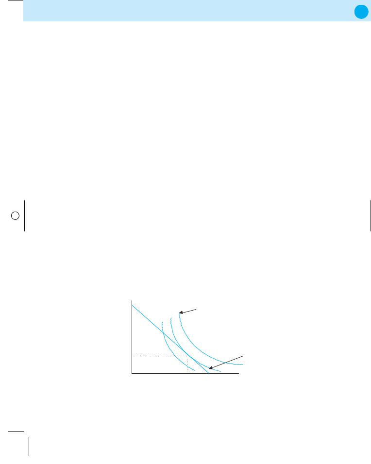
The foregoing analysis can be further examined making reference to Income and Substitution effects, as mentioned in Chapter 2. The income limits facing consumers can be presented using a graphical tool called the budget constraint, which shows the different combinations of goods that can be purchased with a set income, given prevailing prices.
A consumer’s preferences can be illustrated using another graphical tool, the indifference curve, which illustrates various consumption combinations of two goods, which generate the same utility for a consumer. These tools are presented in Figure 3.2 using the information from Tables 3.3 and 3.4. Since the consumer has an income of £200 and the prices of credit or a night out are £50, the maximum amount of either good that could be purchased is 4 units, reflected in the budget line/constraint.
The indifference curve has a curved shape because of the diminishing marginal utility from consuming additional units of each good. The more of one good being consumed, say nights out, the lower the marginal utility from additional consumption of that good. If a consumer consumes many nights out, they would be willing to forego a night out for some call credit, and when little call credit is
Call |
4 |
IC3 |
Indifference curves (IC) |
|
credit |
||||
|
|
IC2 |
|
|
|
|
IC1 |
|
|
|
3 |
|
|
|
|
2 |
|
|
|
|
1 |
|
x |
Budget line/constraint |
|
|
|
|
|
|
1 |
2 |
3 |
Nights out |
|
4 |
|||
F I G U R E 3 . 2 B U D G E T L I N E A N D I N D I F F E R E N C E |
||||
C U R V E A N A L Y S I S |
|
|
|
|

88 |
T H E E C O N O M I C S Y S T E M |
consumed, its marginal utility is high. This is why different combinations of credit and nights out on the indifference curve give rise to the same level of utility.
At different points on the indifference curve, the consumer is willing to trade different amounts of call credit for nights out reflecting the marginal rate of substitution of the goods. This is also reflected in the slope of the indifference curve at any point.
Consumers have a set or map of indifference curves, each with the same shape, that reflect their preferences. Each indifference curve refers to one specific level of utility. On indifference curve IC3 , the consumer has a higher utility level than on IC2 or IC1. Rational consumers attempt to maximize their utility which is equivalent to a desire to consume on the highest possible indifference curve. The actual consumption decision results from preferences indicated by the set of indifference curves and limited income represented by the budget line.
In line with our earlier observation, the consumer in Figure 3.2 chooses to consume 3 nights out and 1 unit of call credit with income of £200, prices of £50 for both goods and given their preferences. Consumption is at point x on IC2 .
The indifference curves drawn for this consumer lie closer to the nights out axis than the call credit axis, which indicates this consumer’s tastes. Another consumer may prefer fewer nights out relative to call credit (if they are new to an area, have not yet made too many friends and prefer to chat to friends back home).
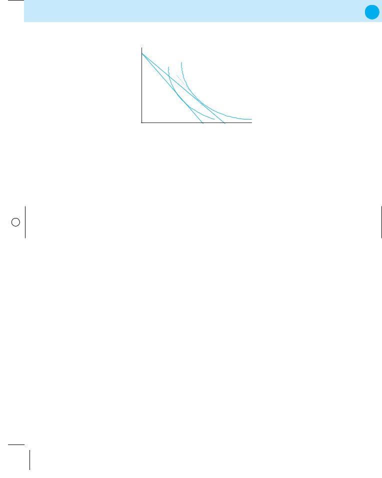
The consumer’s demand decision changes with a price change. If the price of a night out rises to £60, then the maximum number that could be purchased with £200 is 3.3 (£200/60 = 3.33). The budget line changes as shown in Figure 3.3 and consumption moves from x to y. The steeper slope of the line indicates that following the price rise, more call credit must be sacrificed, in opportunity cost terms, to afford one night out. The consumer’s decision to change their quantity demanded of both goods can be broken down into a substitution effect and an income effect.
A price change induces consumers to change their demand decisions. The substitution effect indicates the adjustment in quantity demanded by a consumer due to the change in relative prices alone.
The income effect reflects the adjustment in quantity demanded due to the change in real income alone.
The substitution effect can be examined by considering the price effect alone on the consumer’s choice. To see this we draw a line with the same slope as the new

B E Y O N D D E M A N D : C O N S U M E R S I N T H E E C O N O M I C S Y S T E M |
89 |
Credit |
|
|
|
|
4 |
|
|
|
|
|
IC1 |
IC2 |
|
|
3 |
|
|
|
|
2 |
|
y |
z |
|
|
|
x |
|
|
|
|
|
|
|
1 |
|
|
|
|
|
|
|
|
Nights out |
1 |
2 |
3 |
3.33 |
4 |
F I G U R E 3 . 3 C O N S U M P T I O N W I T H N E W B U D G E T L I N E
budget line and examine where it intersects the original indifference curve IC2 . In Figure 3.3, this occurs at point z.
The substitution effect is measured from x to z. The change in relative prices alone leads to a reduction in quantity demanded of nights out but an increase in the quantity demanded of call credit. The rational consumer substitutes away from the relatively more expensive good towards the relatively cheaper good.
The income effect involves examining the effect on quantity demanded of the reduction in real income caused by the price rise in one good holding relative prices constant. It is shown by the comparison of point z with point y where the same relative prices are used, reflected in the same slope of the two lines. Less of both goods are consumed at point y on IC1 compared to point z on IC2 . The increased price reduces the consumer’s purchasing power and is reflected in reduced demand for all goods, not simply for the good which has become more expensive. This is the pure income effect of the price rise for one good, a normal good.
Normal good: one for which demand falls if real income falls or for which demand rises if income rises.
Inferior good: one for which demand rises if real income falls or for which demand falls if real income rises.
Inferior goods are bought when consumers do not have the required purchasing power to buy other preferred goods. Examples would be many of the goods bought by low-income households – cheaper cuts of meat, non-brand items, etc. The pure income effect of a price fall leads to increased purchasing power and an increase in demand for all normal goods, which are most goods.

90 |
T H E E C O N O M I C S Y S T E M |
C O N S U M E R P R E F E R E N C E S
Where do our preferences come from? Parents, school, friends, experience, advertising? Interesting new research has revealed that neuromarketing – brain scanning via electroencephalogram mapping and functional magnetic-resonance imaging – can be used to analyse consumers’ purchasing decisions and reveal how preferences feed into purchasing decisions.
Neuromarketing is particularly useful for explaining the value of branding. Blind taste tests repeatedly put Pepsi ahead of Coke, which shows up in brain scans that identify greater response of ‘reward centres’ in the brain to Pepsi. Yet Pepsi is not the brand leader. In non-blind taste tests, where subjects were told which cola they were tasting, Coke won out.
Such consumer behaviour was explained in terms of the strength of its brand in the minds of the subjects, which was evident in activity in another area of the brain associated with thinking and judging.
If such thinking and judging activity can be stimulated and influenced by advertising, for example, companies will be able to shape our preferences more clearly! Such research is in its infancy but holds interest for anyone interested in processes that create and change our preferences.
Before we get too carried away with such tests, it has also been pointed out that there is a clear difference between a taste test using a small quantity of product and consuming a larger quantity. Specifically in the cola example, the immediate sugar ‘reward’ from drinking Pepsi is apparently much higher and is preferred in taste tests for this reason. Drinking more than a taste changes the consumer’s perception and the product is found ‘too sweet’ by a majority of the population – no neuromarketing explanation required.
3 . 5 D E M A N D , C O N S U M E R S
A N D C O N S U M E R S U R P L U S
Since consumer satisfaction is examined by means of utility, it should be possible to consider the satisfaction of more than one person in isolation. A problem arises though because utility is subjective and while it is possible to consider one person’s preferences, by asking them to rank them and try to quantify the satisfaction derived from consumption, it is impossible to sum up the satisfaction of more

B E Y O N D D E M A N D : C O N S U M E R S I N T H E E C O N O M I C S Y S T E M |
91 |
Price |
|
|
150 |
|
|
100 |
|
S |
75 |
|
|
50 |
|
|
|
|
D |
18 |
27 |
Quantity (000) |
36 |
F I G U R E 3 . 4 D E M A N D F O R C A L L C R E D I T A N D C O N S U M E R S U R P L U S
than one consumer or try to rank their different preferences. Economists try to get around this problem by means of moving analysis from utility to demand, in the knowledge that the sum of individuals’ consumption choices (based on their marginal utilities) are revealed in the demand for any good. (Economists also use community indifference curves as approximations for the preferences that may be gauged for a group of individuals, despite the difficulties involved.)
Consider the demand for call credit shown in Figure 3.4, with supply included also. Given demand and supply as shown, the equilibrium in the call credit market is for 36 000 units at £50 per unit (the single consumer considered in earlier analysis is just one buyer in the market). The demand at this price is the result of the decisions of many different individuals based on their derived utility from consuming call credit, and their marginal utility/price ratios.
The overall satisfaction generated by the equilibrium consumption can be estimated using the concept of consumer surplus.
Consumer surplus – the benefit to consumers due to the difference between what consumers actually pay to consume a good and what they would have been willing to pay.
In Figure 3.4, although the equilibrium price is £50, many people are willing to pay a higher price. At a price of £75, 27 000 units are demanded while at a price of £100, 18 000 units are in demand. In fact the area under the demand function and above the price provides an estimate of the value of satisfaction generated from consumption of this product (shown as the shaded triangle). The area of this triangle is computed as £1.8 million (the area of a triangle is half the base × perpendicular height which here is 18 000 × 100 = 1 800 000). This indicates the estimated value of the satisfaction generated from the consumption of equilibrium call credit.
