


12.3 Optical Parametric Oscillator with Di racting Pump |
181 |
12.3.1 Turing Instability in a DOPO
An initial comparison with the Turing system suggests that a LALI instability might be observed in a DOPO when the ratio between the pump (inhibitor) and subharmonic (activator) di raction coe cients a reaches a critical value [8].
We proceed again by analyzing the stability of the homogeneous solution of (12.22) against space-dependent perturbations of the form δA(r, t) exp(λt+ik ·r), where δA = (δA0, δA0, δA1, δA1). The resulting linear matrix leads to a fourth-order polynomial in the eigenvalues and then to explicit (although lengthy) analytical expressions for the growth rate λ(k).
In Fig. 12.5 we represent the real part of λ as a function of the perturbation wavenumber k, for three di erent values of the di raction parameter and a fixed positive value of the signal detuning. The parameters are such that an o -resonance instability does not occur (the signal detuning is positive). For zero pump di raction, a = 0 (dotted curve), the homogeneous solution is stable. The o -axis modes are strongly damped, and no LALI instability occurs. For a di raction parameter a = 1/2 (dashed curve in Fig. 12.5), corresponding to the plane-mirror configuration, the homogeneous solution is still stable; the o -axis modes are damped, but the damping around some wavenumbers is weak. This corresponds to a situation where a LALI instability is detectable, but below the threshold (an underdeveloped LALI instability). If the value of the di raction parameter is increased, the largest of the real parts of the eigenvalues grows, until it becomes positive at a critical wavenumber k = kc. This situation is shown by the continuous curve in Fig. 12.5, obtained for a di raction parameter a = 10.
Fig. 12.5. Real part of the eigenvalue as a function of the perturbation wavenumber, for di erent values of the di raction parameter: a = 0 (dotted curve), a = 0.5 (dashed curve) and a = 10 (solid curve). The other parameters are ω1 = 1, ω0 = 0, E = 2.5
182 12 Turing Patterns in Nonlinear Optics
At the threshold of the pattern-forming instability, the real part of the eigenvalue of the wavenumber with maximum growth is zero. In Fig. 12.6, the o -resonance and LALI instability regions are plotted in the parameter space (ω1, E) for a specific value of the di raction parameter. The regions are well separated in the parameter space, and therefore can be associated with di erent mechanisms. The o -resonance instability exists for all values of the pump intensity above threshold, whereas the LALI instability appears only at some critical pump value that depends on the di raction parameter a.
Fig. 12.6. Instability regions in the parameter space (ω1, E) for nonzero di raction parameter a = 5, evaluated from a linear stability analysis. There are two instability regions: for negative detuning, the traditional o -resonance instability; for positive detuning, the Turing instability
We note that pump di raction not only creates the LALI instability, but also modifies the o -resonance instability range, as can be seen from Fig. 12.6. For zero pump di raction the o -resonance instability occurs between the dashed curve and the left part of the solid curve corresponding to the neutral-stability line, as follows from the standard analysis. Pump di raction increases significantly the o -resonance instability region. However, the spatial scale of the o -resonance pattern is not modified by the presence of pump di raction.
Another important feature that reveals the di erent nature of the patterns on both sides of the resonance is the corresponding wavelength. In the case of o -resonance patterns, this wavelength depends mainly on the resonator detuning and the di raction coe cient of the signal wave. In contrast, the wavelength of the pattern in the LALI region depends essentially on the pump and on the ratio of the di raction coe cients a, and very weakly on the resonator detuning. This behavior is shown in Fig. 12.7, where the squared wavenumber of the maximally growing mode is plotted against the detuning (full line). The broken part of the curve, in the neighborhood of the resonance, corresponds to negative eigenvalues.
Some analytical expressions can be found in di erent limits. For negative detuning, the wavenumber is given by
k2 = −ω1 , |
(12.23) |

12.3 Optical Parametric Oscillator with Di racting Pump |
183 |
6 |
|
|
|
|
|
|
k2 |
|
|
|
|
|
|
4 |
|
|
|
|
|
|
2 |
|
|
|
|
|
|
0 |
-4 |
-2 |
0 |
2 |
4 |
6 |
-6 |
||||||
|
|
|
|
|
ω1 |
|
Fig. 12.7. The wavenumber of the pattern, given by a linear stability analysis for a = E = 10. The exact value is given by the solid line. The dashed lines correspond to analytical expressions given in the text
which clearly corresponds to the o -resonance patterns selected by the cavity. For positive detuning,
k2 = |
ω1 |
+ |
2E |
. |
(12.24) |
|
|
||||
|
a |
|
aω1 |
|
|
The asymptotic expressions (12.23) and (12.24) are represented by dashed curves in Fig. 12.7, to be compared with the exact result (full line).
Turing patterns were found by numerical integration of (12.22). In Fig. 12.8 we show the threshold for the emergence of spatial patterns, for a fixed value of signal detuning. Results obtained from the linear stability analysis described above (full line) are shown, together with numerical results for some values of the di raction parameter (represented by symbols). In all cases, the final LALI patterns have hexagonal symmetry, such as the one shown in the
Fig. 12.8. Critical pump value for Turing instability as a function of the di raction parameter, for fixed signal detuning ω1 = 2. The symbols represent the result of numerical integration of the DOPO equations. The solid curve represents the result of a semianalytical calculation based on a linear stability analysis, and the dashed curve corresponds to the boundary of the instability domain given by (12.27). The inset shows a hexagonal pattern obtained numerically for a = 5, E = 3

184 12 Turing Patterns in Nonlinear Optics
inset of Fig. 12.8. For comparison, the preferred patterns occurring in the o -resonance region are not hexagons, but stripes.
The threshold condition for a LALI instability can be evaluated analytically, but is in general a complicated function of the parameters. However, Fig. 12.8 indicates two main features: (i) there exists a hyperbolic relation between the pump and di raction parameters, and (ii) a minimum value of the di raction parameter am is required to reach the instability for a fixed detuning. This guided our search for an asymptotic expression, where we introduced a smallness parameter related to the deviation from the thresh-
old, given by E0 = 1 + ω21. Assuming that R = E0 (E − E0) ≈ O(ε) and D = a − am ≈ O(1/ε), and expanding the eigenvalue, we find, at leading
order in ε, that the homogeneous solution is unstable whenever
27D2R2 − ω12 (2DR − 1)3 < 0 . |
(12.25) |
The minimum value of the di raction parameter am, which depends on the detuning, can be evaluated by analyzing the opposite limit, i.e. at large values of the pump parameter above the threshold. In this case we find that the instability can be observed only when a > am, where
am (E0 − 1) = 1 . |
(12.26) |
From (12.26) it follows that am grows monotonically when the detuning is |
|||
decreased, and that a > 1 (and consequently a0 > a1) when ω1 < |
√ |
|
|
|
3. |
||
Finally, the instability domain (12.25) in the original variables is |
|||
(a − am) (E − E0) < η , |
(12.27) |
||
where η is a positive function of the signal detuning. In the limit of small detuning, (12.25) yields an asymptotic value η = 27/8ω21.
The expression (12.27) is plotted in Fig. 12.8 (as the dashed line) for ω1 = 2 (for which η = 2). Notice the good correspondence with the exact (full line) and numerical (symbols) results.
12.3.2 Stochastic Patterns
The Turing instability in a DOPO occurs only for nonzero signal detuning, as follows from the stability analysis and also from (12.25). However, in resonance, some transverse wavenumbers are weakly damped for nonzero pump di raction. The wavenumber of the weakly damped modes can be obtained from a linear stability analysis of (12.22). In the limit of far above the threshold (E 1), this wavenumber is given by
k2 = |
|
|
2a |
, |
(12.28) |
|
|
|
E |
|
|
12.3 Optical Parametric Oscillator with Di racting Pump |
185 |
which is valid also for small values of the detuning ω1, where pattern formation is expected.
Equation (12.28) corresponds to a ring of weakly damped wavevectors, in the spatial Fourier domain. To check the existence of the ring numerically one must introduce a permanent noise. We can expect that the homogeneous solution will then be weakly modulated by a filtered noise, with a characteristic wavenumber given by (12.28).
In order to incorporate the noise, we have modified (12.22) by adding a term √γiΓi to the evolution equation for each field component Ai. These terms, introduced phenomenologically, represent stochastic Langevin forces defined by
|
Γ |
(r , t |
) |
|
Γ (r , t |
) |
|
= |
δ(r1 − r2)δ(t1 − t2) |
, |
(12.29) |
|
i |
1 |
1 |
i |
2 |
2 |
|
2Ti |
|
||||
where Ti are the corresponding temperatures.
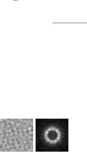
A typical result of numerical integration of the Langevin equations is shown in Fig. 12.9, where a snapshot of the amplitude and the corresponding
2| k |
averaged spatial power spectrum A( ) are shown. As expected, no spatial wavenumber selection was visible in the case of zero pump di raction. For nonzero pump di raction, the DOPO filters the o -axis noise components, and a ring emerges in the far field (Fig. 12.9, right). If the pump di raction parameter is increased, the induced wavenumber ring decreases in radius and becomes more dominant, in accordance with (12.28).
The above calculations were performed for zero detuning for both waves. Therefore all possible pattern formation mechanisms due to o -resonance excitation are excluded.
The expression (12.28) for the wavenumber, although evaluated at resonance, is a good approximation to the wavenumber of the patterns for moderate values of the signal detuning, and corresponds to a characteristic length of the emerging pattern Lp = kc−1. Returning to the initial normalizations of
Fig. 12.9. Stochastic spatial distribution (left) and averaged spatial Fourier power spectrum (right) obtained by numerical integration of the DOPO Langevin equations, for ω1 = 0, E = 2, a0 = 0.005, a1 = 0.0005 (a = 10). The averaging time was t = 300. The zero spectral component has been removed

186 12 Turing Patterns in Nonlinear Optics
the spatial variables in (12.22), this length can be expressed as
Lp2 = |
|
|
|
(12.30) |
|
2E , |
|||
|
|
a0a1 |
|
|
which, together with (12.27), is strikingly similar to the conditions derived in [9] for the Brusselator, a paradigmatic model of chemical pattern formation.
Clearly, the scale of the pattern given by (12.30) depends on the di raction coe cients of both fields. It is interesting to compare the scale of the Turing pattern with the characteristic scales of the components, given by their spatial evolution in the absence of interaction. For this purpose, we consider first a deviation from the trivial solution, A0 = E + X, A1 = Y . In the resonant case and neglecting the nonlinear interaction, (12.22a) leads to
−Y + EY + ia1 2Y = 0 , |
(12.31) |
or, equivalently,
|
a1 |
2 |
|
|
|
|
|
||
1 − |
|
2 |
Y = 0 . |
(12.32) |
E |
||||
Similarly, from (12.22b) we find |
|
|||
−X + ia0 2X = 0 . |
(12.33) |
|||
From the solutions of (12.32) and (12.33), we can define a characteristic spatial scale for the activator, La = a1/E, and for the inhibitor, Li = √a0, corresponding to the signal and pump fields, respectively. Now the scale of the generated pattern can be written in terms of the scales of the activator and the inhibitor, as
|
LaLi |
|
(12.34) |
Lp2 |
= √2 |
, |
revealing that the characteristic spatial scale of the pattern is the geometric mean of the spatial scales of the interacting components.
It is possible to find a simple relation between La and Li in the limit of a am and E E0 (large di raction and pump parameters, and moderate detuning). In this case, the instability domain (12.27) takes the form aE > η, which can be expressed in terms of the characteristic lengths to give the threshold condition
Li > √ |
|
|
(12.35) |
ηLa . |
|||
The value of η depends on the signal detuning and can be evaluated from (12.25)√. We find that η > 1/2 always and, in particular, that η > 1 for ω1 < 3 3. Therefore, for small (and also moderate) detuning, the inhibitor range must be larger than the activator range for the occurrence of the LALI

12.3 Optical Parametric Oscillator with Di racting Pump |
187 |
instability. This is in accordance with the assumptions made in the derivation of (12.28).
The conditions defined by (12.34) and (12.35) are typically found in reaction–di usion systems, and are a signature of the Turing character of the instabilities described above.
12.3.3 Spatial Solitons Influenced by Pump Di raction
The spatial modulation induced by pump di raction also influences the stability of solitons [10], in accordance with the results of Chap. 11. In order to show this, we performed a numerical integration of the DOPO equations (12.22) for di erent values of a0. The amplitude along a line crossing the center of a soliton is plotted in Fig. 12.10, showing that the di raction enhances the spatial oscillations strongly.
The parameters that define the shape of a soliton are the exponent of the spatial decay and the wavenumber of the oscillating tails. These parameters can be analytically evaluated by means of a spatial stability analysis. We assume that the intensity of the field is perturbed from its stationary value in some place in the transverse space (owing to the e ects of boundaries, a spatial perturbation or a defect in the patterns), and look at how this perturbation decays (or grows) in space. For this purpose, we consider evolution in space instead of time. When the system has reached a stationary state, the solution, which we assume to have radial symmetry, can be written in the time-independent form
|
¯ |
(12.36) |
|
Ai = Ai + δAi(r) , |
|
|
2.0 |
|
|
1.0 |
|
A1 |
0.0 |
|
|
-1.0 |
|
|
-2.0 |
x |
|
|
Fig. 12.10. Amplitude profile of a soliton across a line crossing its center, evaluated numerically for di erent pump di raction coe cients, a0 = 0.0005, 0.002 and 0.01. The amplitude of the modulation of the tails increases with increasing di raction. The other parameters are a1 = 0.001, E = 2, ω1 = −0.6, ω0 = 0

188 12 Turing Patterns in Nonlinear Optics
¯
where Ai represents the stationary homogeneous solution for the pump and signal fields, given in (11.2).
After substitution of (12.36) in (12.22), if we consider regions in space not close to the domain boundary, the resulting system can be linearized in the deviation, and the spatial evolution can be described by the system
2 δA = L δA , |
(12.37) |
where δA is the four-component perturbation vector and L is a linear matrix. In the case of a resonant pump, i.e. ω0 = 0, L is given by [10, 11]
|
−i/a |
|
0 |
− (2i/a) A¯1 |
|||
L = |
|
0 |
i/a |
|
|
0 |
|
|
|
¯ |
0 |
|
i (1 + iω1) |
||
|
iA1 |
− |
|||||
|
|
|
|
|
|
|
|
|
|
|
|
|
|
|
|
|
|
0 |
|
¯ |
|
|
¯ |
|
|
− |
iA1 |
|
− |
iA0 |
|
|
|
|
|
|
|
||
(2i/a) A¯1 |
. |
(12.38) |
¯ |
|
|
iA0 |
|
|
i (1 − iω1)
The solutions of the linear system (12.37) are of the form
δA(r) eqr , |
(12.39) |
where the wavevector q can be complex, in the form q |
= Re(q) +i Im(q). |
From (12.39), it follows that a negative value of Re(q) indicates a spatial decay of the perturbation and is responsible for localization, while a nonvanishing value of Im(q) indicates the presence of a nonmonotonic (oscillatory) decay [12]. Thus, the solution (12.36), with the deviation given by (12.39), represents the asymptotic profile of the soliton far from its core.
Expressions for the spatial decay and modulation follow from a study of the eigenvalues of L, which are the solutions of the characteristic equation
a2µ4 −2a2ω1µ3 +(1 − 4aI1) µ2 −2ω1 (1 − 2aI1) µ+4I1 (1 + I1) = 0 , (12.40)
where I1 = A21. Comparing with the ansatz (12.40), we identify q = õ.
A simple analytical solution of (12.40) exists in the case of a resonant
signal, i.e. ω1 = 0, only, and can be written as |
|
|||
|
1 |
−1 + 4aI1 |
± 1 + 8a (2a + 1) I1 . |
|
aµ2 |
= √2 |
(12.41) |
||
We see from (12.41) that the size of the soliton depends on the di raction ratio a in a nontrivial way. This is in contrast with previous studies of pattern formation in many nonlinear optical systems (the Lugiato–Lefever approach [13]), where di raction appears simply as a scale factor in the wavevector, in the form ak2.

12.3 Optical Parametric Oscillator with Di racting Pump |
189 |
In Fig. 12.11 a comparison between analytical results (dashed curve) and numerical results (continuous curve) for the spatial oscillations of the decaying tail of a domain boundary is given. The peak of the localized structure is omitted. Note that the correspondence is very good, even close to the domain boundary (the line of zero intensity). In this particular case, four minima of the intensity are visible. The opposite segment of a dark ring can be locked by each of the minima. Obviously, the soliton of minimum size, locked by the first maximum, which is the strongest, is the most stable one. However, dark rings with larger radii can also be stable.
|
0.0 |
|
|
-0.5 |
|
A1 |
-1.0 |
|
|
-1.5 |
|
|
-2.0 |
r |
|
|
Fig. 12.11. Spatial oscillations of the field outside a soliton, as evaluated numerically (continuous line) and analytically from the spatial stability analysis (dashed line), for E = 2.5, ω1 = 0.5, ω0 = 0, a1 = 0.00025 and a0 = 0.00125 (a = 5)
The stability range of solitons is limited on one hand by the contraction and annihilation of domains, and on the other hand by either the presence of modulational instabilities (the modulations grow, and fill the whole space) or expansion of domains. Since modulational instabilities are favored by di raction, it may seem that di raction has a negative e ect on the stability of solitons. However, for pump values at which instabilities are absent, the increase in the modulation of the tails could prevent full contraction, thus contributing to an enhancement of the stability range. Numerical calculations performed for a large pump di raction parameter show that the stability is always enhanced, at least up to some value of the pump parameter.
The presence of strong modulations in the tails also allows the formation of more complex structures, in the form of bound states of single solitons, or “molecules” of light. Some examples of molecules of varying complexity are shown in Fig. 12.12. Examples with two and three maxima are shown in Figs. 12.12a,b, and a chain composed of five maxima is shown in Fig. 12.12c.

190 12 Turing Patterns in Nonlinear Optics
a) |
b) |
c) |
|
|
|
Fig. 12.12. Several bound states (molecules) of solitons, obtained for a = 5, E = 2.5, ω1 = 0.5, ω0 = 0 : (a) Double; (b) triple; (c) a chain. The field amplitude along a cross section y = 0 of the chain is shown the graph by the solid line. The dashed line represents a section across the space outside the dark line
The internal structure of the chain shown in Fig. 12.12c is more clearly visible in a section along the middle (y = 32). Five maxima at equidistant points are seen. The field along a line outside the domain boundary is given by the dashed line, evaluated at y = 20.
In all cases, the large value of the pump di raction parameter is responsible for the stability of such complex structures, by amplifying the spatial oscillations and thus preventing their collapse. To show this, we have followed the evolution of the soliton “molecules” shown in Figs. 12.12b,c by decreasing the di raction parameter to a = 1 while keeping the other parameters unchanged. The resulting scenario is shown in Fig. 12.13, where the pictures have been taken at equally spaced times. The final state corresponds to a single soliton.