

10.2 Spatial Solitons |
141 |
If the pump power is increased, the real part of the eigenvalue decreases, vanishing at a threshold value p = pmod, where
|
ω2 |
2 |
2 |
|
|
|
1 |
|
|
||
pmod = |
|
24 − 8ω0ω1 + ω0 |
ω1 |
. |
(10.7) |
2 |
For p > pmod, the homogeneous solution is stable. Since pmod is always larger than the pump value given by the upper limit of (10.3) for an arbitrary detuning value, the trivial and modulated solutions coexist in the whole bistability domain. We therefore expect soliton formation in this parameter region.
The bifurcation diagram of the homogeneous solution is depicted in Fig. 10.1.
0.3 |
|
|
Ah stable |
|
|
A |
Ah unstable |
|
| |
|
|
0.2 |
|
|
pmod |
|
|
|
|
|
|
|
|
0.1 |
|
|
|
|
|
0.0 |
0.5 |
1.0 |
1.5 |
2.0 |
2.5 |
0.0 |
|||||
|
|
|
|
|
p |
Fig. 10.1. Bifurcation diagram of homogeneous solution, for ω0 = 10, ω1 = 1. The trivial solution is stable for p < 0.5
10.2 Spatial Solitons
From the viewpoint of soliton formation, an important di erence between the DOPO and the laser studied in the previous chapter is that the solitons in a DOPO are closely related to a modulational instability, which is absent in the case of a laser with a saturable absorber. To show this and to test the above predictions derived from the order parameter equation (10.1), the mean-field model for a DOPO (3.1) has been numerically integrated. We present the results for one and two transverse dimensions.
10.2.1 One-Dimensional Case
In 1D (representing, for example, a resonator with cylindrical mirrors or a system with a slab waveguide configuration), a roll (or stripe) pattern develops for pump values below pmod, sustained by the homogeneous solution. In Fig. 10.2, several periodic solutions obtained for di erent pump values are
142 10 Subcritical Solitons II: Nonlinear Resonance
6 |
|
|
|
4 |
|
|
|
A2 |
|
|
|
2 |
|
|
|
0 |
|
|
|
0 |
4 0 |
8 0 |
1 2 0 |
|
|
x |
|
Fig. 10.2. Stable rolls on a finite background for di erent pump values: (a) E = 1.4, (b) E = 1.6, (c) E = 2. The other parameters are ω0 = 10, ω1 = 1, a1 = 0.001, a0 = a1/2. Note the dependence of the wavenumber on the pump value
shown. Note that not only the wavenumber depends on the pump value (see (10.5)), but also the amplitude of the modulation.
The modulation depth of the stationary pattern, defined as
C = |
Imax − Imin |
, |
(10.8) |
|
Imax + Imin |
||||
|
|
|
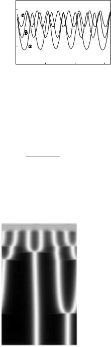
increases with decreasing pump value. At the pump value p = plim, the modulation equals unity (Imin = 0); here the point of zero intensity of the envelope of the roll pattern connects with the trivial solution. Below this pump value, the rolls are no longer stable, and owing to the attracting character of the trivial solution, a dynamical regime appears, shown in Fig. 10.3.
Fig. 10.3. Modulational instability of the homogeneous solution, and soliton formation via annihilation of neighboring solitons. Time runs from top (t = 0) to bottom (t = 75). The pump value is E = 1.2, and the other parameters are as in Fig. 10.2
10.2 Spatial Solitons |
143 |
The initial homogeneous solution is modulationally unstable, and thus in an initial stage a roll pattern emerges, with a wavenumber given by kmax, and with a modulation increasing with time (top part of the figure). Since the pump value is below plim, the roll breaks into independent units, and each of the local maxima of the pattern behaves independently from the others; the maxima interact and merge with their nearest neighbors, and develop into an ensemble of weakly interacting solitons. After a long transient, only one soliton survives.
This scenario of spontaneous soliton formation is not possible in the absence of modulational instability. In the latter case, only localized perturbations strong enough to connecting the two homogeneous branches can lead to soliton formation.
For pump values plim < p < pmod, the solitons are stable, but require a hard localized excitation, as in the case of a laser, as described in the previous chapter.
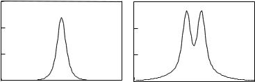
The spatial profile of the solitons is given in Fig. 10.4. Apart from the single soliton usually found (Fig. 10.4a), higher-order solitons can also be stable (although they are less probable). A double-peaked soliton is shown (Fig. 10.4b); this exist in a narrower pump domain. The peak-to-peak distance is close to the width of an individual soliton, and the double-peaked soliton resembles a portion of a periodic pattern.
|
6 |
|
A2 |
4 |
|
|
2 |
|
|
0 |
|
|
x |
x |
Fig. 10.4. Soliton profiles: (a) single, for E = 1.2, and (b) double, for E = 1.35. The other parameters are as in Fig. 10.2
A roll pattern can be interpreted as a periodic array of equally spaced solitons, an idea supported by the numerical results described above (Figs. 10.3 and 10.4). This relation between extended and localized patterns allows estimation of the width of a soliton on the basis of results of a linear stability analysis. To perform this estimation, we consider the asymptotic relations

144 10 Subcritical Solitons II: Nonlinear Resonance
2 2 k x
A ≈ A+ [1 + cos (kx)] ≈ A+ 1 + 1 − 2
= 2A+ 1 − k |
2 |
2 |
≈ 2A+sech |
√2/k |
, |
(10.9) |
|||||||
4x |
|
||||||||||||
|
|
|
|
|
|
|
|
|
|
x |
|
|
|
|
|
|
|
|
|
||||||||
from which the width of the soliton is found to be |
|
||||||||||||
|
√ |
|
|
|
|
|
|
|
|
|
|
|
|
x0 = |
|
2 |
, |
|
|
|
|
|
|
|
|
|
(10.10) |
|
|
|
|
|
|
|
|
|
|
|
|||
|
k |
|
|
|
|
|
|
|
|
|
|||
where k = kmax, given by (10.6).
These results are consistent with an alternative analysis [4, 5], where a parametrically driven Ginzburg–Landau equation was derived as an order parameter equation for the DOPO, under di erent assumptions from those used in the derivation of (10.1). As shown in [5], this equation supports an exact hyperbolic-secant solution, in agreement with the asymptotic solution (10.9).
In Fig. 10.5, the width of the soliton as evaluated numerically (dots) is compared with the analytical value given by (10.10) (full line). Note that the correspondence is better for pump values close to the threshold, in accordance with the assumption made in the derivation of the model (10.1). The dashed lines represent limiting values of the width, those widths corresponding to the largest and smallest wavenumbers that may experience growth (neutrally stable eigenvalues).
3
2
x0
1
0
1.15 1.20 1.25 1.30 1.35
E
Fig. 10.5. Width of the soliton as a function of the pump amplitude. Numerical values (dots) are compared with analytical values (line) derived from the linear stability analysis. Other parameters as in Fig. 10.2
10.2.2 Two-Dimensional Case
The above treatment of 1D solitons can be extended to the 2D case. In 2D, the pattern that coexists with solitons has hexagonal symmetry. Analogously
10.2 Spatial Solitons |
145 |
to the 1D case, below a certain value of the pump, the pattern breaks up into an ensemble of weakly interacting solitons, resembling a “soliton gas”. Neighboring solitons merge, leaving a single soliton after a long transient.
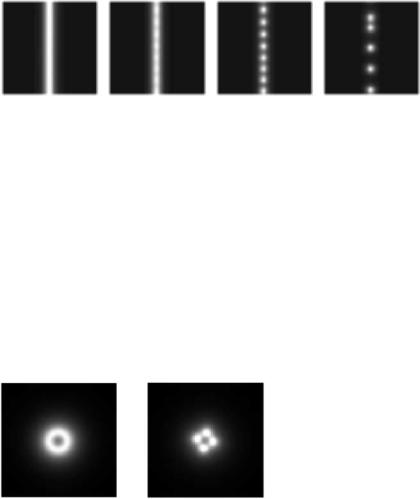
The most straightforward extension of the 1D soliton is a solitary spot. Another extension would be a solitary stripe. However, this kind of soliton is always unstable in 2D, and breaks up into an array of spots which eventually evolve into a single soliton. A scenario of a modulational instability of a localized stripe is shown in Fig. 10.6, where only the initial evolution is shown.
Fig. 10.6. Instability of a localized stripe in two dimensions, and formation of solitons in the form of spots, evaluated at E = 1.3. Other parameters as in Fig. 10.2
The extension of the double soliton to 2D is a localized ring (Fig. 10.7a), and corresponds to Fig. 10.4b in a rotationally symmetric case. If the pump is increased, the ring-shaped soliton can experience a modulational instability in the azimuthal direction, forming an ensemble of single solitons located around the ring (Fig. 10.7b).
More generally, curved solitary lines (of arbitrary shape) in 2D are a ected by modulational instabilities along the direction of the soliton axis, and the straight or circular shapes we have studied are just particular cases.
In conclusion, we have shown that bright spatial solitons can be stable solutions of a model of the degenerate optical parametric oscillator when the pump wave is positively detuned with respect to the closest frequency of the resonator. This result can be explained by noticing the existence of
Fig. 10.7. Higher-order 2D solitons: (a) annular soliton for ω0 = 5; (b) modulated annular soliton for ω0 = 10. Other parameters are E = 1.32 and ω1 = 1