


6.2 Mode Expansion |
93 |
where p = 0, 1, 2, ... is the radial index, and l = ..., −2, −1, 0, 1, 2, ... is the angular index. ρ denotes the radial coordinate normalized to the beam waist r0 = (4a/c)1/4, ϕ is the angle around the optical axis of the laser, and Llp are Laguerre polynomials with the argument indicated. The mode functions are orthonormalized, and obey the condition
2π |
∞ |
|
|
|
|
dϕ |
dρ ρApl(ρ, ϕ)Ap l(ρ, ϕ) = δpp δll . |
(6.5) |
0 |
0 |
|
Alternatively, one can use the Gauss–Hermite mode set; however, for cylindrically symmetric resonators, the Gauss–Laguerre modes are more con-
venient. |
|
The eigenfrequencies of the modes are |
|
√ |
(6.6) |
ωp,l = 2 ac(2p + l + 1) , |
which means that the transverse modes can be degenerate. The fundamental Gaussian mode TEM00 (p = 0, l = 0) has a frequency ω0 = 2√ac; the
two single-vortex helical modes TEM |
(p = 0, l = |
± |
1) have a frequency |
0±1 |
|
|
ω = 2ω0; the next mode family consists of the nonhelical mode TEM10 (p = 1,
l = 0) and two helical double-vortex modes TEM |
(p = 0, l = |
± |
2), and so |
0±2 |
|
|
on. The nth transverse mode family n = 2p + l is n times degenerate.
6.2 Mode Expansion
Modes are eigenfunctions of a linear resonator. In a nonlinear resonator, the modes become coupled. We can then rewrite (6.3) in terms of coupled mode amplitudes, by expanding the order parameter into modes:
A(r, t) = fi(t)Ai(r) , (6.7)
i
where i is an arbitrary combination of mode indices p and l. Inserting the expansion (6.7) into (6.3), multiplying both sides by Aj (r), integrating and taking into account of the orthonormality of the modes, we obtain
∂fi |
|
|
|
= pifi − i(ωi + ω0)fi − Γjkil fj fkfl , |
(6.8) |
∂τ |
||
|
jkl |
|
where pi = p − (ωi + ω0)2κ2 the modes, and Γiljk are the
/(κ + γ )2 are the individual gain coe cients of nonlinear coupling coe cients, given by
Γiljk = Aj (r)Ak(r)Ai (r)Al (r) dr . (6.9)

94 6 Resonators with Curved Mirrors
The mode expansion is not very useful if many modes are taken into account. The computer time required to integrate (6.8) numerically is proportional to the fourth power of the number of modes. Therefore, for a large number of modes, the numerical integration of the partial di erential equation (6.3) is usually more convenient. However, the mode expansion approach is very useful if a small number of modes is excited. The usefulness of mode expansion is illustrated below with two examples of circling vortices, and with an example of transverse-mode locking.
6.2.1 Circling Vortices
Vortices circling around the optical axis of a laser can be interpreted as the interference of two modes of di erent helicities. In this case, (6.8) becomes
|
∂f1 |
= p1f1 − i(ω1 + ω0)f1 − f1(G11 |f1| |
2 |
|
2 |
|
||||
|
|
|
+ 2G12 |
|f2| ) , |
(6.10a) |
|||||
|
∂τ |
|
||||||||
|
∂f2 |
= p2f2 − i(ω2 + ω0)f2 − f2(G22 |f2| |
2 |
|
2 |
|
||||
|
|
|
+ 2G12 |
|f1| ) , |
(6.10b) |
|||||
|
∂τ |
|
||||||||
where |
|
= |
|
|
|
|
|
|
|
|
G11 |
= Γ1111 |
|A1(r)|4 |
dr , |
|
|
|
(6.11a) |
|||
G22 |
= Γ2222 |
= |
|A2(r)|4 |
dr , |
|
|
|
(6.11b) |
||
G12 |
= Γ1212 |
= Γ2121 = |
|A1(r)|2 |A2(r)|2 dr . |
|
(6.11c) |
|||||
From (6.10), one can analyze the behavior of two modes with di erent helicities. For example, it is found that the frequencies of the modes are not a ected by the nonlinear interaction. The particular spatial shapes of the helical modes do not lead to nonlinear mode pulling or locking. The variation of the di erence between the phases of the modes only rotates the two-mode interference pattern around the optical axis of the laser, and consequently there is no preferred phase di erence.
There are several di erent solutions for the intensities of the modes ni = |fi|2. One solution is trivial, with the amplitudes of both modes equal to zero. This solution is, however, unstable if the laser is above the generation threshold. Another solution corresponds to a single mode, where the intensity of one mode is zero, and the intensity of the other is ni = pi/Gii. The most interesting solution is that where both modes are excited,
n1 |
= |
p1G22 − 2p2G12 |
, |
(6.12a) |
|
G11G22 − 4G122 |
|||||
|
|
|
|
||
n2 |
= |
p2G11 − 2p1G12 |
. |
(6.12b) |
|
G11G22 − 4G122 |
|||||
|
|
|
|
6.2 Mode Expansion |
95 |
A stability analysis of these solutions shows that the two modes can coexist (and beat, if they have di erent eigenfrequencies) if G11G22 > 4G212, which means that the modes overlap relatively weakly. For example, the fundamental mode TEM00 and the single-vortex mode TEM01 overlap relatively
strongly and the above inequality is invalid. The overlap between these two
√ √
modes is G12/ G11G22 = 1/ 2, which is larger than the critical overlap of 1/2 for the coexistence of modes. These two modes, therefore, cannot exist simultaneously. Interference of the modes TEM00 and TEM01 results in an optical vortex rotating around the optical axis of the laser. Such behavior is, however, unstable for a class A laser, as (6.12) shows, and either the vortex spirals in and subsequently remains on the optical axis of the laser (the helical TEM01 mode wins the competition), or the vortex spirals out and disappears (the fundamental TEM00 mode wins). A steadily spiraling vortex is possible only in a class B laser, as shown in Chap. 7.
Instead of one single vortex, however, several circling vortices are easily obtained in the framework of (6.11). A number l of vortices of the same charge arranged symmetrically around the optical axis of the laser corresponds to
the interference pattern of a TEM0l mode with the fundamental Gaussian
mode. The mode overlap decreases with increasing l. For example, the overlap
√
between the TEM02 and√TEM00 modes is 1/ 6, that between the TEM03 and TEM00 modes is 1/ 20, and so on.
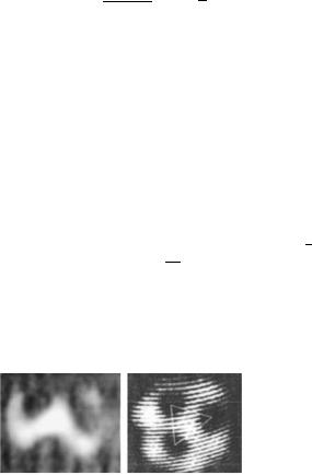
In Fig. 6.2, an example of multiple circling vortices is shown, taken from [2]. Note that while multiple circling vortices are relatively easily obtained experimentally, a single circling vortex following a circular trajectory has never been observed.
Fig. 6.2. Three vortices circling around the optical axis of a laser. At the right, an interference picture with a tilted plane wave is shown. The interference fringes indicate the topological charges of the vortices
6.2.2 Locking of Transverse Modes
Another example concerns the locking of the transverse modes. In this case, instead of helical modes (6.4), a expansion into flowerlike modes is more convenient:
Apli(ρ, ϕ) = √π (2ρ2)1/2 |
(p + l)! |
1/2 |
× |
sin(lϕ), i = 2 , |
||||
Lpl (2ρ2)e−ρ |
||||||||
2 |
|
|
p! |
2 |
|
cos(lϕ), i = 1 |
||
|
|
|
|
|
|
|
|
|
(6.13)
96 6 Resonators with Curved Mirrors
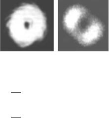
Fig. 6.3. Perfectly locked vortex (left ) and a vortex locked with some nonzero angle between the phases of the “flower” modes of which it is composed (right ). The experiments were done with a photorefractive oscillator
which are also orthogonal and normalized. Taking now two modes from the same transverse mode family, we obtain, instead of (6.11),
∂f∂τ1 = p1f1 − i(ω1 + ω0)f1 − f1(G11 |f1|2 + 2G12 |f2|2) − G12f22f1 ,
(6.14a)
∂f∂τ2 = p2f2 − i(ω2 + ω0)f2 − f2(G22 |f2|2 + 2G12 |f1|2) − G12f12f2 ,
(6.14b)
where the phase-sensitive terms (the last term in the right-hand side) are included. The phase-sensitive coupling coe cient is given by
G12 = Γ2211 = Γ1122 = A21(r)A22(r) dr . (6.15)
The role of the phase-sensitive terms is to lock the frequencies of the two modes (i.e. to synchronize the modes) if their eigenfrequencies do not di er too much. If we restrict our considerations, for simplicity, to the case of symmetric modes (p1 = p2 = p, G11 = G22), the solution of (6.14) is
p |
− |
n [G |
+ 2G |
+ G |
cos (4 ∆ϕ)] = 0 |
, |
|
||||
|
11 |
12 |
|
12 |
|
|
|
|
|||
|
|
|
|
∆ω |
− |
nG |
|
sin (4 ∆ϕ) = 0 |
. |
(6.16) |
|
|
|
|
|
|
|
|
|||||
|
|
|
2 |
|
|
||||||
|
|
|
|
12 |
|
|
|
||||
Here ∆ω = ω1 − ω2 is the frequency mismatch between the two modes, n is the intensity of each of the modes, and ∆ϕ = ϕ1 −ϕ2 is their phase di erence.
The solution (6.16) indicates that the modes lock with the same phase if the frequency detuning is equal to zero. In general, the phase-locking angle is proportional to the detuning. Figure 6.3 (left) shows a perfectly locked vortex and (right) a vortex where the corresponding “flower” modes are locked at a nonzero angle.
Evidently, there exists a maximum value of the mode frequency mismatch for which the modes are still locked,
∆ωthr = |
2pG12 |
(6.17) |
||
|
|
. |
||
G11 |
+ 2G |
|||
|
|
12 |
|
|
Figure 6.4 shows examples of mode-locked patterns involving a small number of modes, obtained experimentally [3].