

Ersoy O.K. Diffraction, Fourier optics, and imaging (Wiley, 2006)(ISBN 0471238163)(427s) PEo
.pdf18 LINEAR SYSTEMS AND TRANSFORMS
When fy ¼ 0,
1ð
Uðfx; 0Þ ¼ ½h2ðxÞ h1ðxÞ&e j 2p fx xdx
1
¼ H2ðfxÞ H1ðfxÞ
Thus, Uðfx; 0Þ is the difference of the 1-D FT of the functions h2ðxÞ and h1ðxÞ.
2.6REAL FOURIER TRANSFORM
Sometimes it is more convenient to represent the Fourier transform with real sine and cosine basis functions. Then, it is referred to as the real Fourier transform (RFT). What was discussed as the Fourier transform before would then be the complex Fourier transform (CFT) [Ersoy, 1994]. For example, the analytic signal representation of nonmonochromatic wave fields can be more effectively derived using the RFT, as discussed in Section 9.4. In this and next sections, we will discuss the 1-D transforms only.
The RFT of a signal uðxÞ can be defined as
|
|
|
1 |
|
|
|
|
Uðf Þ ¼ 2wðf Þ |
ð |
uðtÞ cosð2p ft þ yð f ÞÞdx |
ð2:6-1Þ |
||||
|
|
|
1 |
|
|
|
|
where |
|
|
|
( 1=2 f |
¼6 0 |
|
|
|
wðf Þ ¼ |
ð2:6-2Þ |
|||||
|
|
|
|
1 |
f |
0 |
|
|
|
|
|
|
|
¼ |
|
|
|
|
|
0 |
f |
0 |
|
|
yðf Þ ¼ ( p=2 f < 0 |
ð2:6-3Þ |
|||||
The inverse RFT is given by |
|
|
|
|
|
|
|
|
1 |
|
|
|
|
|
|
uðtÞ ¼ |
ð |
Uð f Þ cosð2p ft þ yð f ÞÞdf |
ð2:6-4Þ |
||||
|
1 |
|
|
|
|
|
|
It is observed that cosð2pft þ yð f ÞÞ equals cosð2pftÞ for f ¼ 0 and sinð2pj f jtÞ for f < 0. This is a ‘‘trick’’ used to cover both the cosine and sine basis functions in a single integral. Negative frequencies are used for this purpose. It is interesting
REAL FOURIER TRANSFORM |
|
|
|
|
|
|
|
|
|
|
|
|
19 |
||||
|
1.5 |
|
|
|
|
|
|
|
|
|
|
|
|
|
|
|
|
|
|
|
|
|
|
|
|
|
|
|
|
|
|
|
|
|
|
|
1 |
|
|
|
|
|
|
|
|
|
|
|
|
|
|
|
|
|
|
|
|
|
|
|
|
|
|
|
|
|
|
|
|
|
|
FunctionBasis |
0.5 |
|
|
|
|
|
|
|
|
|
|
|
|
|
|
|
|
|
|
|
|
|
|
|
|
|
|
|
|
|
|
|
|
||
0 |
|
|
|
|
|
|
|
|
|
|
|
|
|
|
|
|
|
|
|
|
|
|
|
|
|
|
|
|
|
|
|
|
|
|
|
|
–0.5 |
|
|
|
|
|
|
|
|
|
|
|
|
|
|
|
|
|
|
|
|
|
|
|
|
|
|
|
|
|
|
|
|
|
|
|
–1 |
|
|
|
|
|
|
|
|
|
|
|
|
|
|
|
|
|
|
|
|
|
|
|
|
|
|
|
|
|
|
|
|
|
|
|
–1.5 |
|
|
|
|
|
|
|
|
|
|
|
|
|
|
|
|
|
|
–5 |
|
|
|
0 |
|
|
|
5 |
|
|
|
10 |
|||
|
–10 |
|
|
|
|
|
|
|
|
|
|||||||
|
|
|
|
|
Frequency |
|
|
|
|
|
|
|
|
|
|||
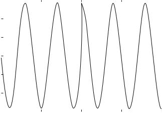
Figure 2.3. |
p2 cos 2 |
ft |
f |
ÞÞ |
for t |
¼ |
0 25 and |
10 |
< |
f |
< |
10. |
|||||
The basis function |
|
ð |
p |
þ yð |
|
: |
|
|
|
|
|||||||
p
to observe that 2 cosð2pft þ yð f ÞÞ is orthonormal with respect to f because Eq. (2.6-4) is true. Thus,
|
1 |
|
|
|
|
|
|
|
|
|
|
|
|
|
|
2 |
ð0 |
cosð2pft þ yð f ÞÞ cosð2pf t þ yð f ÞÞdf ¼ dðt tÞ |
|
|
ð2:6-5Þ |
||||||||||
where dð Þ is the Dirac-delta function. |
|
ÞÞ |
|
¼ |
|
: |
|
||||||||
10 < f < 10. |
|
|
ð |
2 |
p |
ft |
þ yð |
f |
is shown in Figure 2.3 for t |
0 |
25 and |
||||
The basis function p2 cos |
|
|
|
|
|
|
|||||||||
Equations (2.6-1) and (2.6-4) can also be written for f ¼ 0 as |
|
|
|
|
|||||||||||
|
|
|
|
|
|
|
|
|
1 |
|
|
|
|
|
|
|
|
U1ðf Þ ¼ 2wðf Þ |
ð |
uðtÞ cosð2p ftÞdt |
|
|
ð2:6-6Þ |
||||||||
|
|
|
|
|
|
|
|
1 |
|
|
|
|
|
||
|
|
|
|
|
|
|
1 |
|
|
|
|
|
|
|
|
|
|
U0ðf Þ ¼ 2 |
ð |
uðtÞ sinð2p ftÞdt |
|
|
ð2:6-7Þ |
||||||||
|
|
|
|
|
|
|
1 |
|
|
|
|
|
|
|
|
and |
|
|
|
|
|
|
|
|
|
|
|
|
|
|
|
|
|
1 |
|
|
|
|
|
|
|
|
|
|
|
|
|
|
uðtÞ ¼ ð |
½U1ð f Þ cosð2p ftÞ þ U0ð f Þ sinð2p ftÞ&df |
|
|
ð2:6-8Þ |
||||||||||
0

20 LINEAR SYSTEMS AND TRANSFORMS
Thus, Uð f Þ equals U1ð f Þ for f ¼ 0 and X0ðj f jÞ for f < 0. X1ð f Þ and X0ð f Þ will be referred to as the cosine and sine parts, respectively. Equations (2.6-1), (2.6-6), and (2.6-7) are also referred to as the analysis equations. Equations (2.6-4) and (2.6-8) are the corresponding synthesis equations.
The relationship between the CFT and the RFT can be expressed for f 0 as
" Uc |
|
Ucð0Þ ¼ |
Uð0Þ |
j |
#" U0 |
ð f Þ #f > 0 |
ð2:6-9Þ |
|||||
|
ð |
fÞ # |
¼ |
2 " |
1 |
|||||||
Uc |
|
f |
|
1 |
|
1 |
j |
U1 |
f |
|
||
|
ð Þ |
|
|
|
|
|
|
|
ð Þ |
|
||
Equation (2.6-9) reflects the fact that U1ðf Þ and U0ðf Þ are even and odd functions, respectively.
The inverse of Eq. (2.6-9) for f 0 is given by
U1ð0Þ ¼ Ucð0Þ |
|
#" U |
|
cð |
fÞ |
#f > 0 |
ð2:6-10Þ |
||||
" U1 |
ðf Þ # |
¼ |
" j |
|
j |
|
|||||
U |
f |
|
1 1 |
|
U |
f |
|
|
|
||
0 |
ð Þ |
|
|
|
|
|
cð Þ |
|
|
||
Equations (2.6-9) and (2.6-10) are useful to convert from one representation to the other. When xðtÞ is real, U1ðf Þ and U0ðf Þare also real. Then, Eq. (2.6-9) shows that Ucðf Þ and Ucð f Þ are complex conjugates of each other.
2.7AMPLITUDE AND PHASE SPECTRA
Ucðf Þ can be written as
Ucðf Þ ¼ Uaðf Þ e jfðf Þ; |
ð2:7-1Þ |
where the amplitude (magnitude) spectrum Uað f Þ and the phase spectrum fð f Þ of the signal xðtÞ are defined as
|
|
|
|
1 |
hjU1 |
ð f Þj2 þ jU0ð f Þj2i |
1=2 |
|
||
Uað f Þ ¼ jUcð f Þj ¼ |
|
ð2:7-2Þ |
||||||||
2 |
||||||||||
fð |
|
Þ ¼ |
|
Real ½Uc½ð f Þ& |
|
ð |
Þ |
|||
|
f |
|
tan 1 |
Imaginary |
Ucð f Þ& |
|
2:7-3 |
|
||
|
|
|
|
|
|
|
|
|||
Uað f Þis an even function. With real signals, fð f Þ is an odd function and can be written as
fð f Þ ¼ tan 1½ U0ðf Þ=U1ð f Þ& |
ð2:7-4Þ |
HANKEL TRANSFORMS |
21 |
Equation (1.2.2) for the inverse CFT can be written in terms of the amplitude and phase spectra as
|
|
1 |
|
|
uðtÞ ¼ |
ð |
Uað f Þe j½2p ftþfð f Þ&df |
ð2:7-5Þ |
|
|
|
1 |
|
|
When uðtÞ is real, this equation reduces to |
|
|||
|
1 |
|
|
|
uðtÞ ¼ 2 |
ð0 |
Uað f Þ cos½2p ft þ fð f Þ&df |
ð2:7-6Þ |
|
because Ucð f Þ ¼ Uc ð f Þ, and the integrand in
1ð
j Uað f Þ sin½2p ft þ fð f Þ&df
1
is an odd function and integrates to zero.
Equation (2.7-6) will be used in representing nonmonochromatic wave fields in Section 9.4.
2.8HANKEL TRANSFORMS
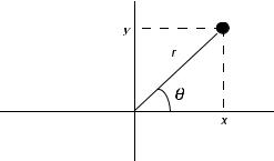
Functions having radial symmetry are easier to handle in polar coordinates. This is often the case, for example, in optics where lenses, aperture stops, and so on are often circular in shape.
Let us first consider the Fourier transform in polar coordinates. The rectangular and polar coordinates are shown in Figure 2.4. The transformation to polar
Figure 2.4. The rectangular and polar coordinates.
22 |
|
|
|
|
LINEAR SYSTEMS AND TRANSFORMS |
||||
coordinates is given by |
|
|
|
|
|
|
|
|
|
|
r ¼ ½x2 þ y2&1=2 |
|
|
|
|||||
|
|
|
y |
|
|
|
|||
|
y ¼ tan 1 |
|
|
|
|
|
|
|
|
|
x |
ð |
2:8-1 |
Þ |
|||||
|
r ¼ ½fx2 þ fy2&1=2 |
|
|||||||
|
f ¼ tan 1 |
|
fy |
|
|
|
|
||
|
fx |
|
|
|
|||||
The FT of uðx; yÞ is given by |
ðð uðx; yÞe j2p ð fxxþfyyÞdxdy |
|
|
|
|||||
Uðfx; fyÞ ¼ |
ð2:8-2Þ |
||||||||
|
1 |
|
|
|
|
|
|
|
|
|
1 |
|
|
|
|
|
|
|
|
f ðx; yÞ in polar coordinates is f ðr; yÞ. Fð fx; fyÞ in polar coordinates is Fð r; fÞ, given by
2p |
1 |
|
|
|
|
|
|
|
Uðr; fÞ ¼ ð0 |
dy ð0 |
uðr; yÞe j2p rrðcos y cos fþsin y sin fÞrdr |
ð2:8-3Þ |
|||||
When uðx; yÞ is circularly symmetric, it can be written as |
|
|||||||
|
|
|
uðr; yÞ ¼ uðrÞ |
ð2:8-4Þ |
||||
Then, Eq. (2.6-3) becomes |
|
|
|
|
|
|
|
|
|
1 |
|
|
|
2p |
|
|
|
Uðr; fÞ ¼ ð0 |
uðrÞrdr ð0 |
e j2prr cosðy fÞdy |
ð2:8-5Þ |
|||||
The Bessel function of the first kind of zero order is given by |
|
|||||||
|
|
|
|
|
2p |
|
|
|
|
J0ðtÞ ¼ |
1 |
ð0 |
e jt cosðy fÞdy |
ð2:8-6Þ |
|||
|
2p |
|||||||
It is observed that J0ðtÞ is the same for all values of f. Substituting this identity in Eq. (2.8-5) and incorporating an extra factor of 2p gives
1ð
Uðr; fÞ ¼ UðrÞ ¼ 2p uðrÞJ0ð2prrÞrdr |
ð2:8-7Þ |
0

HANKEL TRANSFORMS |
23 |
Thus, the 2-D FT of a circularly symmetric function is itself circularly symmetric and is given by Eq. (2.8-7). This relation is called the Hankel transform of zero order or the Fourier-Bessel transform.
It can be easily shown that the inverse Hankel transform of zero order is given by the same type of integral as
1 |
|
|
|
uðrÞ ¼ 2p ð0 |
UðrÞJ0ð2prrÞrdr |
ð2:8-8Þ |
|
|
|
|
|
EXAMPLE 2.5 Derive Eq. (2.8-5). |
|
|
|
Solution: x, y and fx, fy are given by |
|
|
|
x ¼ r cos y |
|
y ¼ r sin y |
|
fx ¼ r cos f |
fy ¼ r sin f |
|
|
Equation (2.8-2) becomes
2p |
1 |
|
Uðr; fÞ ¼ ð0 |
dy ð0 |
uðr; yÞe j2prrðcos y cos fþsin y sin fÞJdr |
where J is the Jacobian given by
|
|
@x |
|
@x |
|
|
|
|
|
|
|
@y |
|
|
cos y |
J |
|
@r |
|
|
|
||
|
|
@r |
|
@y |
|
|
|
|
|
|
|
|
|
|
|
|
|
@y |
|
@y |
|
sin y |
|
|
¼ |
|
¼ |
||||
|
|
|
|
|
|
|
|
r sin y ¼ r r cos y
ð2:8-9Þ
ð2:8-10Þ
where j j indicates determinant. Substituting J ¼ r in Eq. (2.8-9) gives the desired result.
EXAMPLE 2.6 (a) Find the Hankel transform of the cylinder function cylðrÞ defined by
|
|
|
1 |
0 r < |
1 |
|
|
|
||||
|
|
> |
|
|
|
|
|
|||||
|
|
2 |
|
|
|
|||||||
|
|
8 |
|
|
|
|||||||
|
|
> |
|
|
|
|
|
|
|
|
|
|
|
|
> |
|
|
|
1 |
|
|
|
|
|
|
|
|
< |
|
|
|
|
|
|
|
|
|
|
cyl r |
Þ ¼ |
> |
1 |
r |
¼ |
1 |
|
ð |
2:8-11 |
Þ |
||
ð |
> |
2 |
|
2 |
|
|
||||||
|
|
> |
|
|
|
|
|
|
|
|
|
|
|
|
> |
|
|
|
|
|
|
|
|
|
|
|
|
> |
|
|
|
|
|
|
|
|
|
|
|
|
> |
|
|
|
|
|
|
|
|
|
|
|
|
: |
|
|
|
|
|
|
|
|
|
|
|
|
> |
0 |
r > |
2 |
|
|
|
|
|
|
|
(b) Find the Hankel transform of cylðr=DÞ.

24 LINEAR SYSTEMS AND TRANSFORMS
Solution: (a) Let
uðrÞ ¼ cylðrÞ
Then
|
1 |
|
|
|
|
|
|
|
|
|
|
||
UðrÞ ¼ 2p ð uðrÞJ0ð2prrÞrdr |
|
|
|
||||||||||
|
|
0 |
|
|
|
|
|
|
|
|
|
|
|
|
1=2 |
|
|
|
|
|
|
|
|
|
|||
|
|
ð |
|
|
|
|
|
|
|
|
|
|
|
¼ 2p J0ð2prrÞrdr |
|
|
|
||||||||||
|
|
0 |
|
|
|
|
|
|
|
|
|
|
|
The Bessel function of the first kind of first order is given by [Erdelyi] |
|
|
|
||||||||||
|
|
|
1=2 |
|
|
|
|
|
|
||||
J1ðprÞ ¼ 4pr |
ð0 |
J0ð2prrÞrdr |
ð2:8-12Þ |
||||||||||
Hence, |
|
|
|
|
|
|
|
|
|
|
|
|
|
U |
ðrÞ ¼ |
|
J1ðprÞ |
|
|
|
|
||||||
|
|
|
|
2r |
|
|
|
||||||
The sombrero function sombðrÞ is defined by |
|
|
|
||||||||||
somb |
r |
Þ ¼ |
2J1ðprÞ |
ð |
2:8-13 |
Þ |
|||||||
|
pr |
||||||||||||
|
ð |
|
|
|
|||||||||
UðrÞ is related to sombðrÞ by |
|
|
p |
|
|
|
|
|
|
|
|||
|
|
|
|
|
|
|
|
|
|
||||
UðrÞ ¼ |
|
sombðrÞ |
|
|
|
||||||||
4 |
|
|
|
||||||||||
(b) We have |
|
|
|
|
|
|
|
|
|
|
|
|
|
|
|
|
D=2 |
|
|
|
|
|
|
|
|||
U0ðrÞ ¼ 2p ð0 |
|
J0ð2prrÞrdr |
|
|
|
||||||||
Let r0 ¼ r=D. Then, dr ¼ Ddr0, and |
|
|
|
|
|
|
|
|
|
|
|
|
|
|
|
1=2 |
|
|
|
|
|
|
|
|
|
||
U0ðrÞ ¼ 2pD2 |
|
ð0 |
|
r0J0ð2prDrÞdr0 |
|
|
|
||||||
2 |
|
|
|
|
|
|
|
D2p |
|
|
|
||
¼ D UðrÞ ¼ |
|
|
sombðDrÞ |
|
|
|
|||||||
|
4 |
|
|
|
|||||||||
|
|
|
|
|
|
|
|
|
|
|
|
|
|

3
Fundamentals of Wave Propagation
3.1INTRODUCTION
In this chapter and Chapter 4, waves are considered in 3-D, in general. However, in some applications such as in integrated optics in which propagation of waves on a surface is often considered, 2-D waves are of interest. For example, see Chapter 19 on dense wavelength division multiplexing. Two-dimensional equations are simpler because one of the space variables, say, y is omitted from the equations. Hence, the results discussed in 3-D in what follows can be easily reduced to the 2-D counterparts.
Electromagnetic (EM) waves will be of main concern. They are generated when a time-varying electric field Eðr; tÞ produces a time-varying field Hðr; tÞ. EM waves propagate through unguided media such as free space or air and in guided media such as an optical fiber or the medium between the earth’s surface and the ionosphere. In this chapter, we will be mainly concerned with unbounded media.
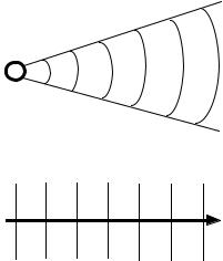
Spherical waves result when a source such as an antenna emits EM energy as shown in Figure 3.1(a). At a far away distance from the source, the spherical wave appears like a plane wave with uniform properties at all points of the wavefront, as seen in Figure 3.1(b). Another example would be an electric dipole directed along the z-axis, located at the origin, and oscillating with the circular frequency w. It generates electric and magnetic fields with a complicated expression, but far from the origin where the fields look like plane waves. A perfect plane wave does not exist physically, but it is a component that is very useful in modeling all kinds of waves.
Waves propagate in a medium. In the case of optical waves, the optical medium is characterized by a quantity n called the refractive index. It is the ratio of the speed of light in free space to that of the speed of light in the medium. The medium is homogeneous if n is constant, otherwise, it is inhomogeneous. In this chapter, we will assume that the medium is homogeneous.
The chapter consists of seven sections. How waves come about and some of their fundamental properties are discussed in Section 3.2. The fundamental properties of EM waves and the Kirchoff equations that characterize them are discussed in Section 3.3. The phasor representation is reviewed in Section 3.4. Wave equations,
Diffraction, Fourier Optics and Imaging, by Okan K. Ersoy
Copyright # 2007 John Wiley & Sons, Inc.
25
26 |
FUNDAMENTALS OF WAVE PROPAGATION |
Source
(a)
Propagation
Direction
(b)
Figure 3.1. (a) Spherical wave generated by a source; (b) plane wave with uniform properties along the direction of propagation.
the wave equation in a source free medium as well as the plane wave solution with wave number and direction cosines, are described in Section 3.5. Wave equations in phasor representation in a charge-free medium are discussed in Section 3.6. Plane waves are fundamental components of EM waves. They are described in more detail in Section 3.7, including their polarization properties.
3.2WAVES
Nature is rich in a large variety of waves, such as electromagnetic, acoustical, water, and brain waves. A wave can be considered as a disturbance of some kind that can travel with a fixed velocity and is unchanged in form from point to point.
Let uðx; tÞ denote a 1-D wave in the x-direction in a homogeneous medium. If v is its velocity, uðx; tÞ satisfies
uðx; tÞ ¼ uðx vt; 0Þ |
ð3:2-1Þ |
if it is traveling to the right and
uðx; tÞ ¼ uðx þ vt; 0Þ |
ð3:2-2Þ |
if it is traveling to the left.
Assuming the wave is traveling to the left, let s be given by
s ¼ x þ vt |
ð3:2-3Þ |

WAVES |
27 |
Then, the following can be computed:
|
|
|
@u |
¼ |
@u |
|
|
|
|
|||||||
|
|
|
@x |
|
@s |
|
|
|
|
|
|
|
|
|
||
|
|
@2u |
¼ |
@2u |
|
|
|
|
|
|||||||
|
|
@x2 |
|
@s2 |
|
|
|
|
||||||||
|
|
|
@u |
|
@s @u |
|
@u |
|||||||||
|
|
|
|
¼ |
|
|
|
|
|
|
¼ v |
|
|
|||
|
|
|
@t |
|
@t @s |
@s |
||||||||||
|
|
@2u |
¼ v2 |
@2u |
||||||||||||
|
|
@t2 |
@s2 |
|
|
|
|
|||||||||
Hence, |
|
|
|
|
|
|
|
|
|
|
|
|
|
|||
@2uðx; tÞ |
|
|
|
1 @2uðx; tÞ |
||||||||||||
|
|
|
@x2 |
|
¼ |
v2 |
|
|
@t2 |
|||||||
ð3:2-4Þ
ð3:2-5Þ
This equation is known as the nondispersive wave equation. A particular solution, which is also a solution for all other wave equations, is the simple harmonic solution given by
x
ðx; tÞ ¼ A cosðkðx þ vtÞÞ ¼ A cosðkx þ wtÞ ¼ A cos 2p l þ ft ; ð3:2-6Þ
where o ¼ 2pf and k ¼ 2p=l. l is the wavelength, f is the time frequency, 1=l is the spatial frequency, and o and k are the corresponding angular frequencies. k is also known as the wave number. ðx; tÞ given by Eq. (3.2-6), is also known as the 1-D plane wave.
Because of mathematical ease, Eq. (3.2-6) is often written as
uðx; tÞ ¼ Re½AejðkxþotÞ& |
ð3:2-7Þ |
|||||
or simply as |
|
|
|
|
|
|
u |
x; t |
Þ ¼ |
AejðkxþotÞ |
ð |
3:2-8 |
Þ |
ð |
|
|
|
|||
‘‘real part’’ being understood from the content. We reassert that the wave number k is the radian spatial frequency along the x-direction. It can also be written as
k ¼ 2pfx |
ð3:2-9Þ |
where fx is the spatial frequency in the x-direction in cycles/unit length. Substituting Eq. (3.2-8) into Eq. (3.2-5) gives
v ¼ |
o |
ð3:2-10Þ |
k |