Mueller M.R. - Fundamentals of Quantum Chemistry[c] Molecular Spectroscopy and Modern Electronic Structure Computations (Kluwer, 2001)

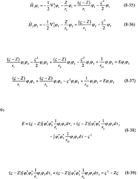
Substituting Equations 8-35 and 8-36 into Equation 8-34 results in the following expression.

Equation 8-37 is now multiplied by and integrated over all space. This results in the following expression due to the orthonormality of and

The first two integrals in Equation 8-38 correspond to the average Coulombic potential energy of each electron with the nucleus.

The third integral in Equation 8-38 is the electron-electron repulsion potential. This is the same as the integral that was solved previously in the perturbation theory method (see Equations 8-27 through 8-32) except now Z is replaced with

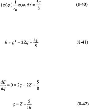
Equations 8-39 and 8-40 can now be substituted into Equation 8-38 resulting in an energy expression in terms of the adjustable parameter

Now that an energy expression has been obtained in terms of the effective nuclear charge an optimal value for must be determined by minimizing the energy.

For a helium atom so the effective nuclear charge is equal to 27/16. Physically this means that the electrons experience a nuclear charge of 27/16 rather than 2. If the optimized value of for helium is substituted into the Equation 8-41, the energy eigenvalue for the ground-state of helium is -2.85 eV which is in relatively good agreement with experiment.

The perturbation and variational approach to solving for the energy of a helium atom demonstrates that the hydrogen atom wavefunctions are not a good starting point for solving the Schroedinger equation of atoms with multiple electrons. The electron-electron repulsion potential has a profound affect on the energy of a system with multiple electrons, as it has been determined for the case of the helium atom. The charge of the nucleus experienced by the electrons is reduced as a result of shielding, and some of the degeneracy of the orbitals is lost. A better set of functions as a basis set for solving systems with multiple electrons will be discussed in Section 8.4.

The electrons in an atom also have an intrinsic angular momentum in addition to their orbital angular momentum about the nucleus. This is called the electron spin or sometimes just referred to as spin. Even an electron in the orbital that has zero angular momentum will have an intrinsic spin. The intrinsic spin of the electron is not a classical mechanical effect; hence, it is not a correct picture to view the electron spinning about one of its axes, as the classical mechanical picture would indicate. The term “spin” is more of a name for this phenomenon rather than an actual description of the electron. Though the intrinsic spin of the electron is real, there is no example in the macroscopic world to form a visual model. The electron spin arises naturally when relativistic mechanics is combined with quantum mechanics. Since this text is confined to quantum mechanics, the concept of electron spin must be introduced as a hypothesis.

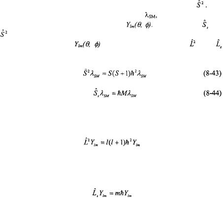
Since an electron has an intrinsic spin, there must be a corresponding

Equation 8-43 is the analog of the equation for overall orbital angular momentum squared.

Equation 8-44 is the analog to the equation for the z-component of orbital angular momentum.

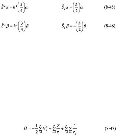
There are only two possible values for the M and S quantum numbers for a single electron (such as in a hydrogen atom): +½ or -½. The eigenfunction for the eigenstate is given the symbol and is called “spin up”. The eigenstate is given the symbol and is called “spin down”.

The complete designation for a hydrogen atom wavefunction will include the intrinsic spin eigenstate:

The Pauli principle states that no two electrons in an atom or molecule can occupy the same spin-orbital. This means that for an atom, each spatial orbital (e.g. and so on) can have only two electrons and they must be of opposite spin. This adds a two-fold degeneracy to each spatial orbital for an atom or a molecule.

8.4 COMPLEX ATOMS

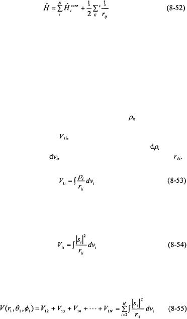
The Hamiltonian for an atom with N electrons, ignoring nuclear motion, can be written as follows.

The first term in the Hamiltonian corresponds to the kinetic energy of each electron, the second term is the Coulombic attraction of each electron to the nucleus with an atomic number Z, and the third term is the Coulombic repulsion between each electron. The index j > i in the summation prevents terms such as

The zeroth-order wavefunction, as in the case for the helium atom, will be a product of N-one-electron functions.

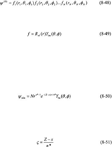
The general form of the functions f will be a radial function, times a spherical harmonic function,

One possibility as a basis set of functions to be used for f is the hydrogenatom functions. As seen in the case of a helium atom, this is not a particularly good start. The hydrogen-atom wavefunctions do not account for shielding and other affects of the inter-electronic repulsion. A basis set of functions that take this into account is a much better starting point for the calculation. J. C. Slater created such a basis set of functions known as the Slater-type orbitals (STO). The functions have the following general form.

The term s is the shielding constant and n* is a parameter that varies with the principal quantum number n. The term N is the radial normalization constant. The effective nuclear charge, can be calculated from s and n * as follows.

The Slater-type orbitals replace the polynomial in r as in hydrogenlike orbitals with a single power in r reducing computational effort. The values for s and n* are determined empirically by the following procedure.

1.The electrons of the atom are put into the following groups.

{1s}; {2s, 2p}; {3s, 3p}; {3d}; {4s, 4p}; {4d}; {4f}; {5s, 5p}; ...

2.There is no contribution to screening, s, from any electron within a given group.

3.In the 1s group, the contribution to s is 0.30. For electrons outside the 1s group, the contribution to s is 0.35 for each electron in that group.

4.For an electron in an s or p orbital, the contribution to s is 0.85 for each other electron when the principal quantum number n is one less than for the orbital being written. For still lower levels of n, the contribution to s is 1.00.

5.For electrons in d and f orbitals, the contribution to s is 1.00 for each electron below the one for which the wavefunction is being written.

6.The value for n * is determined based on the value for n as follows.

Example 8-4

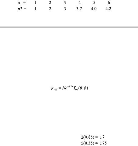
Problem: Determine the Slater-type orbital wavefunction and for an electron in a) the ground-state of helium, and b) the orbital of oxygen.

Solution:

a) For helium, The only screening is from the other electron so value for The value of so the value for The Slater-type orbital wavefunction for a helium atom in the ground-state is as follows.

The effective nuclear charge is 1.7, the same value as obtained previously from variational theory in Section 8.2.

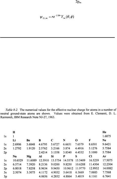
b) For oxygen, For an electron in the orbital, and so The contributions to the screening constant s are summed as follows.

2 electrons in the 1s orbital:

5 electrons in 2s and 2p orbitals:

The effective nuclear charge for an electron in a orbital in oxygen is 2.28.

There are several deficiencies in STO’s. Because STO’s replace the polynomial in r for a single term, STO’s do not have the proper number of nodes and do not represent the inner part of an orbital well. Care must be taken when using STO’s because orbitals with the different values of n but the same values of l and are not orthogonal to one another. Another deficiency is that ns orbitals where n > 1 have zero amplitude at the nucleus. Values have been obtained for the effective nuclear charge for a number of atoms by fitting STO’s to numerically computed wavefunctions. These values are given Table 8-2 and supersede the values obtained empirically from Slater’s rules.

Solving the Schroedinger equation for an atom with N electrons is a formidable computational task because of the numerous electron-electron repulsion terms, In order to calculate the electron repulsion of one electron, the wavefunctions for the other electrons must be known and viceversa. The best atomic orbitals are obtained by a numerical solution of the Schroedinger equation. The procedure first introduced by D.R. Hartree is called self-consistent field (SCF). The procedure was further improved by including electron exchange by V. Fock and J.C. Slater. The orbitals obtained by a combination of these procedures are called Hartree-Fock selfconsistent field orbitals.

The Hartree-Fock self-consistent field (HF-SCF) approach assumes that any one electron moves in a potential that is a spherical average due to the other electrons and the nucleus. The spherically averaged potential for an electron is expressed as a single charge that is centered on the nucleus and varies with the position r in the potentially averaged sphere. The Schroedinger equation is then numerically solved for that electron in the spherically averaged potential. Of course in order to determine the spherically averaged potential for a particular electron, the wavefunctions (and hence relative positions) of the other electrons must be known. Since the wavefunctions of the other atoms is most likely not known, the calculations begin with approximate wavefunctions as a basis set for the other electrons such as STO’s. The wavefunction is assumed to be a product of one-electron wavefunctions as in Equation 8-48. The result of this assumption is that the electrons in the atom are ordered in hydrogenlike orbitals. As an example, the electrons in oxygen are ordered in the familiar fashion of The Schroedinger equation is then solved for the electron, and then the procedure is repeated for the rest of the electrons in the atom. After this first computation, a set of improved wavefunctions as the basis set for the electrons is obtained. The computation is now repeated with this new set of wavefunctions for each electron. A new set of wavefunctions is obtained for each electron and is compared to wavefunctions from the previous computational cycle. If the values are different, a new computational cycle is performed with the latest wavefunctions obtained for the electrons. If the wavefunctions do not differ significantly from the previous computational cycle, the computation is complete and the wavefunctions are said to be self-consistent.

The details of a HF-SCF computation can now be examined in detail. In the HF-SCF approach, the Hamiltonian for an atom is written in terms of a summation of hydrogenlike terms plus the electron repulsion terms.

The term is called the core Hamiltonian and represents the electron i in a potential that consists of only the nucleus of atomic number Z with no repulsive potential from any other electron (as in a one-electron system). The factor of ½ is to eliminate counting the same electron-electron repulsions twice. The prime is a reminder not to count any terms.

The focus is now on electron 1, and the rest of the electrons (2, 3, 4, ..., N) are regarded as being distributed about to form part of the spherically

electron per unit volume) that electron 1 travels through. The potential of

The probability density of the electrons is given as As a result, the charge density of an electron is given as

The potential interaction of electron 1 with all N electrons are determined and summed together.