You must distinguish between the primary index and secondary indexes of a table. The primary index contains the key fields of the table. The primary index is automatically created in the database when the table is activated. If a large table is frequently accessed such that it is not possible to apply primary index sorting, you should create secondary indexes for the table.

Indexes of a table have a three-place index ID. 0 is reserved for the primary index. Customers can create their own indexes on SAP tables; their IDs must begin with Y or Z.

If the index fields have key function, for example, they already uniquely identify each record of the table, an index can be called a unique index. This ensures that there are no duplicate index fields in the database.

When you define a secondary index in the ABAP Dictionary, you can specify whether it should be created on the database when it is activated. Some indexes only result in a gain in performance for certain database systems. You can therefore specify a list of database systems when you define an index. The index is then only created on the specified database systems when activated.

Improving the Performance through Table Buffering

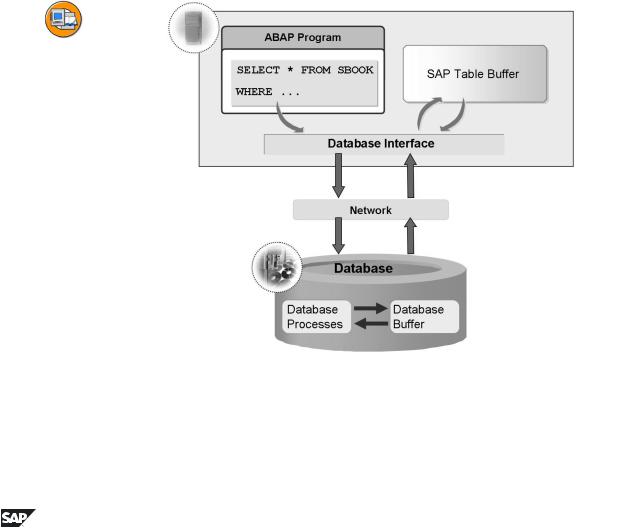
Figure 32: Data Access using the Buffer

Table buffering increases the performance when the records of the table are read.

The records of a buffered table are read directly from the local buffer of the application server on which the accessing transaction is running when the table is accessed. This eliminates time-consuming database accesses. The access improves by a factor of 10 to 100. The increase in speed depends on the structure of the table and on the exact system configuration. Buffering, therefore, can greatly increase the system performance.

If the storage requirements in the buffer increase due to further data, the data that has not been accessed for the longest time is displaced. This displacement takes place asynchronously at certain times which are defined dynamically based on the buffer accesses. Data is only displaced if the free space in the buffer is less than a predefined value or the quality of the access is not satisfactory at this time.

When you enter /$TAB in the command field the system resets the table buffers on the corresponding application server. Only use this command if there are inconsistencies in the buffer. In large systems, it can take several hours to fill the buffers. The performance is considerably reduced during this time.

The buffering type determines which records of the table are loaded into the buffer of the application server when a record of the table is accessed. There are the following buffering types:

•Full buffering: When a record of the table is accessed, all the records of the table are loaded into the buffer.

•Generic buffering: When a record of the table is accessed, all the records whose left-justified part of the key is the same are loaded into the buffer.

•Single-record buffering: Only the record that was accessed is loaded into the buffer.

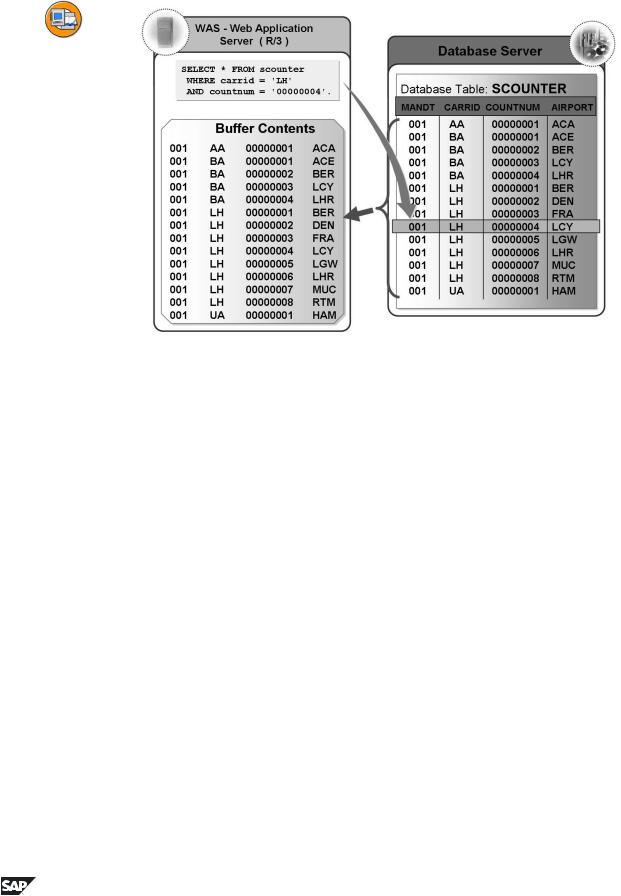
Figure 33: Full Buffering

With full buffering, the table is either completely or not at all in the buffer. When a record of the table is accessed, all the records of the table are loaded into the buffer.

When you decide whether a table should be fully buffered, you must take the table size, the number of read accesses and the number of write accesses into consideration. The smaller the table is, the more frequently it is read and the less frequently it is written, the better it is to fully buffer the table.

Full buffering is also advisable for tables that have frequent accesses to records that do not exist. Since all the records of the table reside in the buffer, it is already clear in the buffer whether or not a record exists.

The data records are stored in the buffer sorted by table key. When you access the data with SELECT, only fields up to the last specified key field can be used for the access. The left-justified part of the key should therefore be as large as possible for such accesses. For example, if the first key field is not defined, the entire table is scanned in the buffer. Under these circumstances, a direct access to the database could be more efficient if there is a suitable secondary index there.

Figure 34: Generic Buffering

With generic buffering, all the records whose generic key fields agree with this record are loaded into the buffer when one record of the table is accessed. The generic key is a left-justified part of the primary key of the table that must be defined when the buffering type is selected. The generic key should be selected so that the generic areas are not too small, which would result in too many generic areas. If there are only a few records for each generic area, full buffering is usually preferable for the table. If you choose too large a generic key, too much data will be invalidated if there are changes to table entries, which would have

a negative effect on the performance.

A table should be generically buffered if only certain generic areas of the table are usually needed for processing.

Client-dependent, fully buffered tables are automatically generically buffered. The client field is the generic key. It is assumed that not all of the clients are being processed at the same time on one application server. Language-dependent tables are a further example of generic buffering. The generic key includes all the key fields up to and including the language field.

The generic areas are managed in the buffer as independent objects. The generic areas are managed analogously to fully buffered tables. You should therefore also read the information about full buffering.

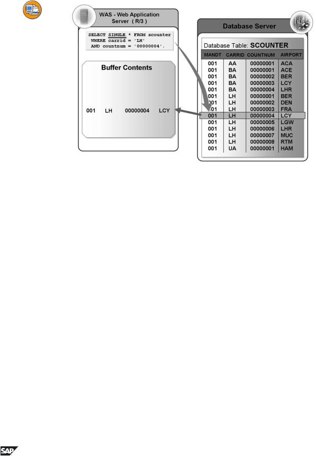
Figure 35: Single-Record Buffering

Only those records that are actually accessed are loaded into the buffer. Single-record buffering saves storage space in the buffer compared to generic and full buffering. The overhead for buffer administration, however, is higher than for generic or full buffering. Considerably more database accesses are necessary to load the records than for the other buffering types.

Single-record buffering is recommended particularly for large tables in which only a few records are accessed repeatedly with SELECT SINGLE. All the accesses to the table that do not use SELECT SINGLE bypass the buffer and directly access the database.

If you access a record that was not yet buffered using SELECT SINGLE, there is a database access to load the record. If the table does not contain a record with the specified key, this record is recorded in the buffer as non-existent. This prevents a further database access if you make another access with the same key.

You only need one database access to load a table with full buffering, but you need several database accesses with single-record buffering. Full buffering is therefore generally preferable for small tables that are frequently accessed.

Figure 36: Table buffering

The R/3 System manages and synchronizes the buffers on the individual application servers. If an application program accesses data of a table, the database interfaces determines whether this data lies in the buffer of the application server. If this is the case, the data is read directly from the buffer. If the data is not in the buffer of the application server, it is read directly from the database and loaded into the buffer. The buffer can therefore satisfy the next access to this data.

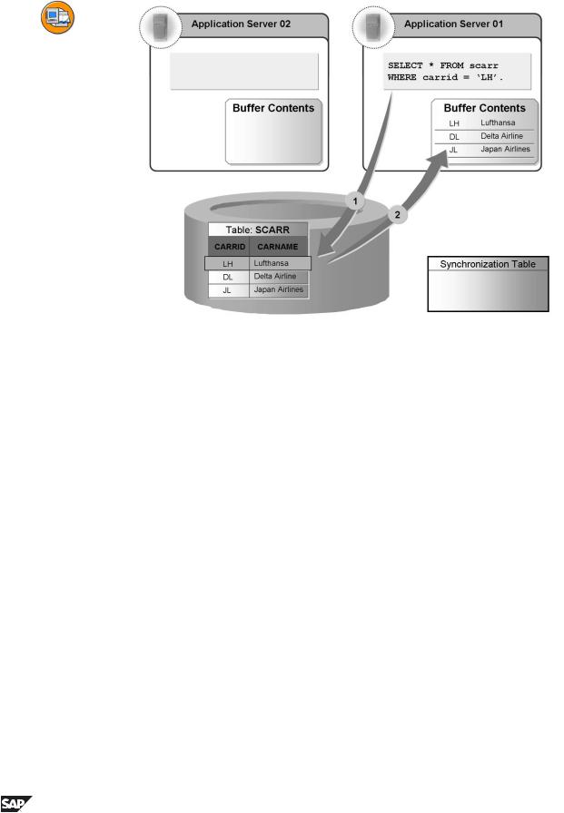
Figure 37: Buffer Synchronization 1

Since the buffers reside locally on the application servers, they must be synchronized after data has been modified in a buffered table. Synchronization takes place at fixed time intervals that can be set in the system profile. The corresponding parameter is “rdisp/bufreftime” and defines the length of the interval in seconds. The value must lie between 60 and 3600. We recommend a value between 60 and 240.

The following example shows how the local buffers of the system are synchronized. A system with two application servers is assumed.

•Timepoint 1: Server 1 reads records from table SCARR on the database.

•Timepoint 2: Table SCARR is fully loaded into the local buffer of Server 1. The local buffer of this server is now used for access from Server 1 to the data of the SCARR table.

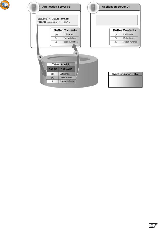
Figure 38: Buffer Synchronization 2

•Timepoint 3: A user on Server 2 accesses records of the table. Since the table does not yet reside in the local buffer of Server 2, the records are read directly from the database.

•Timepoint 4: The SCARR table is loaded into the local buffer of Server 2. Server 2 therefore also uses its local buffer to access its data when it next reads the SCARR table.

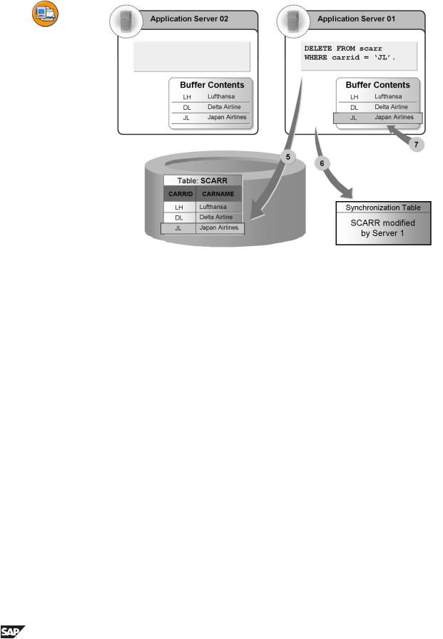
Figure 39: Buffer Synchronization 3

•Timepoint 5: A user on Server 1 deletes records from the SCARR tyble and updates the database.

•Timepoint 6: Server 1 writes an entry in the synchronization table.

•Timepoint 7: Server 1 updates its local buffer.

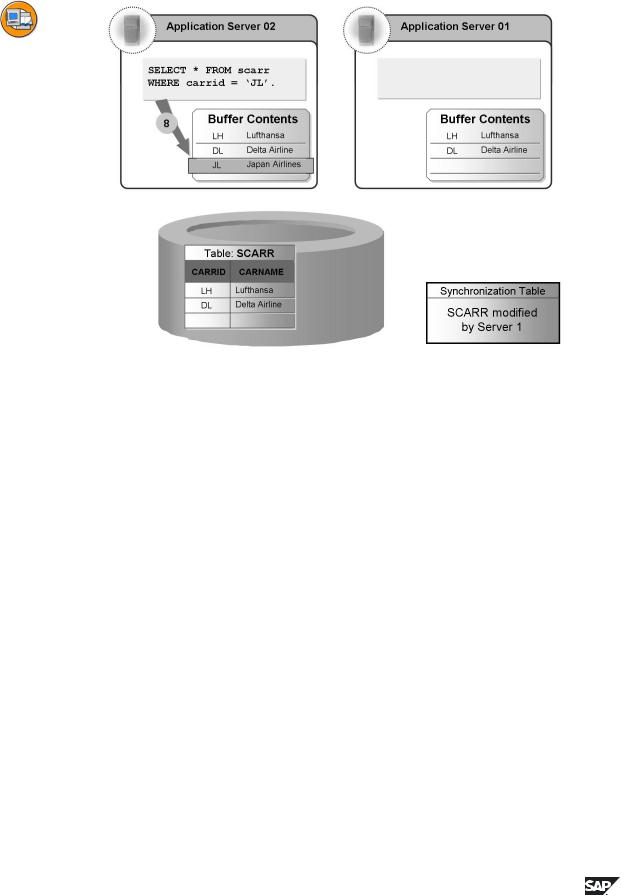
Figure 40: Buffer Synchronization 4

•Timepoint 8: A user on Server 2 accesses the deleted records. Since the SCARR table resides in its local buffer, the access uses this local buffer.

–Server 2 therefore finds the records although they no longer exist in the database table.

–If the same access were made from an application program to Server 1, this program would recognize that the records no longer exist. At this time the behavior of an application program depends on the server on which it is running.

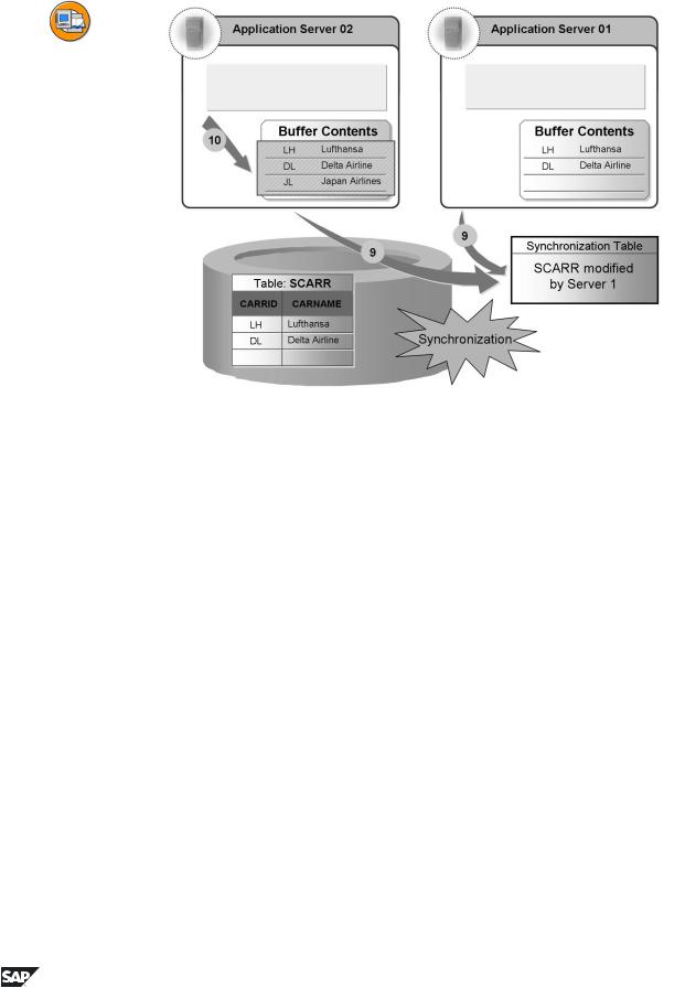
Figure 41: Buffer Synchronization 5

•Timepoint 9: The moment of synchronization has arrived. Both servers look in the synchronization table to see if another server has modified one of the tables in its local buffer in the meantime.

•Timepoint 10: Server 2 finds that the SCARR table has been modified by Server 1 in the meantime. Server 2 therefore invalidates the table in its local buffer. The next access from Server 2 to data of the SCARR table therefore uses the database. Server 1 must not invalidate the table in its buffer, as it is the only changer of the SCARR table itself. Server 1 therefore uses its local buffer again the next time to access records of SCARR table.

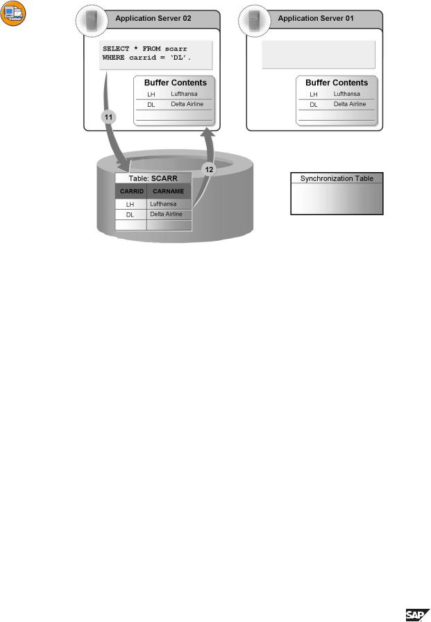
Figure 42: Buffer Synchronization 6

•Timepoint 11: Server 2 again accesses records of SCARR table. Since SCARR is invalidated in the local buffer of Server 2, the access uses the database.

•Timepoint 12: The table is reloaded into the local buffer of Server 2. The information via the SCARR table is now inconsistent again on the servers and the database.

Advantages and disadvantages of this method of buffer synchronization:

•Advantage: The load on the network is kept to a minimum. If the buffers were to be synchronized immediately after each modification, each server would have to inform all other servers about each modification to a buffered table via the network. This would have a negative effect on the performance.

•Disadvantage: The local buffers of the application servers can contain obsolete data between the moments of synchronization.

This means that:

•Only those tables that are written very infrequently (read mostly) or for which such temporary inconsistencies are of no importance may be buffered.

•Tables whose entries change frequently should not be buffered. Otherwise there would be a constant invalidation and reload, which would have a negative effect on the performance.

An index helps you to speed up read accesses to a table. An index can be considered a sorted copy of the table that is reduced to the index fields.

The table buffers reside locally on the application servers.

Buffering can substantially increase the performance when the records of the table are accessed. Choosing the correct buffering type is important.

The table buffers are adjusted to changes to the table entries at fixed intervals.

The more frequently a table is read and the less frequently the table contents are changed, the better it is to buffer the table.

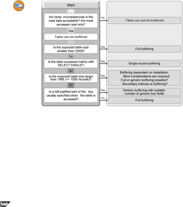
Figure 43: Decision Tree for Buffering

The decision-making tree for buffering tables should be used for support on your development system. The information mentioned above is shown here as a diagram.