CHAPTER

EIGHT

CURVE FITTING

One of the most important tasks in any experimental science is modeling data and determining how well some theoretical function describes experimental data. In the last chapter, we illustrated how this can be done when the theoretical function is a simple straight line in the context of learning about Python functions and methods. Here we show how this can be done for a arbitrary fitting functions, including linear, exponential, power law, and other nonlinear fitting functions.

8.1Using linear regression for fitting non-linear functions

We can use our results for linear regression with 2 weighting that we developed in Chapter 7 to fit functions that are nonlinear in the fitting parameters, provided we can transform the fitting function into one that is linear in the fitting parameters and in the independent variable (x).

8.1.1 Linear regression for fitting an exponential function

To illustrate this approach, let’s consider some experimental data taken from a radioactive source that was emitting beta particles (electrons). We notice that the number of electrons emitted per unit time is decreasing with time. Theory suggests that the number of electrons N emitted per unit time should decay exponentially according to the equation

141

Introduction to Python for Science, Release 0.9.23

This equation is nonlinear in t and in the fitting parameter and thus cannot be fit using the method of the previous chapter. Fortunately, this is a special case for which the fitting function can be transformed into a linear form. Doing so will allow us to use the fitting routine we developed for fitting linear functions.

We begin our analysis by transforming our fitting function to a linear form. To this end we take the logarithm of Eq. (8.1):

t ln N = ln N0 :

With this tranformation our fitting function is linear in the independent variable t. To make our method work, however, our fitting function must be linear in the fitting parameters, and our transformed function is still nonlinear in the fitting parameters and N0. Therefore, we define new fitting parameters as follows

a = ln N0

(8.2)

b = 1=

Now if we define a new dependent variable y = ln N, then our fitting function takes the form of a fitting function that is linear in the fitting parameters a and b

y = a + bx

where the independent variable is x = t and the dependent variable is y = ln N.

We are almost ready to fit our transformed fitting function, with transformed fitting parameters a and b, to our transformed independent and dependent data, x and y. The last thing we have to do is to transform the estimates of the uncertainties N in N to the uncertainties y in y (= ln N). So how much does a given uncertainty in N translate into an uncertainty in y? In most cases, the uncertainty in y is much smaller than y, i.e. y y; similarly N N. In this limit we can use differentials to figure out the relationship between these uncertainties. Here is how it works for this example:

y = ln N

@y

Equation (8.3) tells us how a small change N in N produces a small change y in y. Here we identify the differentials dy and dN with the uncertainties y and N. Therefore, an uncertainty of N in N corresponds, or translates, to an uncertainty y in y.

Introduction to Python for Science, Release 0.9.23

Let’s summarize what we have done so far. We started with the some data points fti; Nig and some addition data f Nig where each datum Ni corresponds to the uncertainty in the experimentally measured Ni. We wish to fit these data to the fitting function

N(t) = N0e t= :

We then take the natural logarithm of both sides and obtain the linear equation

t

ln N = ln N0 (8.4) y = a + bx

with the obvious correspondences

x = t

y = ln N

(8.5)

a = ln N0 b = 1=

Now we can use the linear regression routine with 2 weighting that we developed in the previous section to fit (8.4) to the transformed data xi(= ti) and yi(= ln Ni). The inputs are the tranformed data xi; yi; yi. The outputs are the fitting parameters a and b, as well as the estimates of their uncertainties a and b along with the value of 2. You can obtain the values of the original fitting parameters N0 and by taking the differentials of the last two equations in Eq. (8.5):

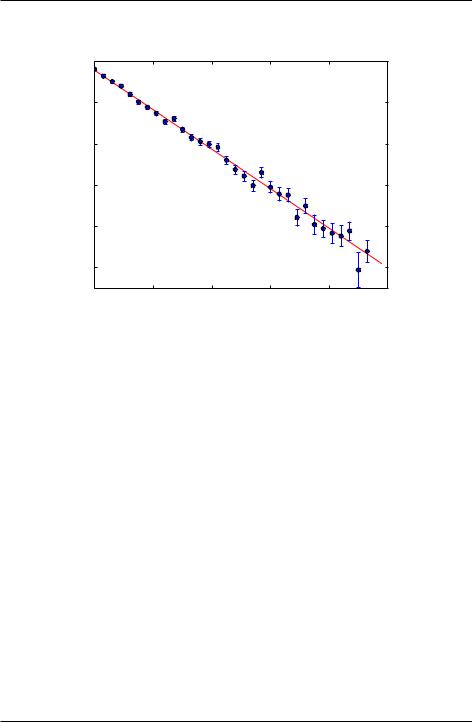
Figure 8.1 shows the output of the fit to simulated beta decay data obtained using the program below. Note that the error bars are large when the number of counts N are small. This is consistent with what is known as shot noise (noise that arises from counting discrete events), which obeys Poisson statistics. You will study sources of noise, including shot noise, later in your lab courses. The program also prints out the fitting parameters of the transformed data as well as the fitting parameters for the exponential fitting function.

import numpy as np

import matplotlib.pyplot as plt

Introduction to Python for Science, Release 0.9.23

Figure 8.1: Semi-log plot of beta decay measurements from Phosphorus-32.

def LineFitWt(x, y, sig):

"""

Fit to straight line.

Inputs: x and y arrays and uncertainty array (unc) for y data. Ouputs: slope and y-intercept of best fit to data.

"""

sig2 = sig**2

norm = (1./sig2).sum()

xhat = (x/sig2).sum() / norm yhat = (y/sig2).sum() / norm

slope = ((x-xhat)*y/sig2).sum()/((x-xhat)*x/sig2).sum() yint = yhat - slope*xhat

sig2_slope = 1./((x-xhat)*x/sig2).sum() sig2_yint = sig2_slope * (x*x/sig2).sum() / norm

return slope, yint, np.sqrt(sig2_slope), np.sqrt(sig2_yint)

def redchisq(x, y, dy, slope, yint):

chisq = (((y-yint-slope*x)/dy)**2).sum() return chisq/float(x.size-2)

# Read data from data file

Introduction to Python for Science, Release 0.9.23

t, N, dN = np.loadtxt("betaDecay.txt", skiprows=2, unpack=True)

########## Code to tranform & fit data starts here ##########

#Transform data and parameters to linear form: Y = A + B*X X = t # transform t data for fitting (trivial)

Y = np.log(N) # transform N data for fitting

dY = dN/N # transform uncertainties for fitting

#Fit transformed data X, Y, dY to obtain fitting parameters A & B

#Also returns uncertainties in A and B

B, A, dB, dA = LineFitWt(X, Y, dY)

#Return reduced chi-squared redchisqr = redchisq(X, Y, dY, B, A)

#Determine fitting parameters for original exponential function

#N = N0 exp(-t/tau) ...

N0 = np.exp(A) tau = -1.0/B

# ... and their uncertainties dN0 = N0 * dA

dtau = tau**2 * dB

####### Code to plot transformed data and fit starts here #######

#Create line corresponding to fit using fitting parameters

#Only two points are needed to specify a straight line

Xext = 0.05*(X.max()-X.min())

Xfit = np.array([X.min()-Xext, X.max()+Xext])

Yfit = A + B*Xfit

plt.errorbar(X, Y, dY, fmt="bo") plt.plot(Xfit, Yfit, "r-", zorder=-1) plt.xlim(0, 100)

plt.ylim(1.5, 7)

plt.title("$\mathrm{Fit\\ to:}\\ \ln N = -t/\\tau + \ln N_0$") plt.xlabel("t")

plt.ylabel("ln(N)")

plt.text(50, 6.6, "A = ln N0 = {0:0.2f} $\pm$ {1:0.2f}"

.format(A, dA))

plt.text(50, 6.3, "B = -1/tau = {0:0.4f} $\pm$ {1:0.4f}"

.format(-B, dB))

plt.text(50, 6.0, "$\chi_r^2$ = {0:0.3f}"

.format(redchisqr))

Introduction to Python for Science, Release 0.9.23

plt.text(50, 5.7, "N0 = {0:0.0f} $\pm$ {1:0.0f}"

.format(N0, dN0))

plt.text(50, 5.4, "tau = {0:0.1f} $\pm$ {1:0.1f} days"

.format(tau, dtau))

plt.show()

8.1.2 Linear regression for fitting a power-law function

You can use a similar approach to the one outlined above to fit experimental data to a power law fitting function of the form

We follow the same approach we used for the exponential fitting function and first take the logarithm of both sides of (8.7)

We recast this in the form of a linear equation y = a + bx with the following identifications:

x = ln s

y = ln P

(8.9)

a = ln P0 b =

Following a procedure similar to that used to fit using an exponential fitting function, you can use the tranformations given by (8.9) as the basis for a program to fit a power-law fitting function such as (8.8) to experimental data.

8.2 Nonlinear fitting

The method introduced in the previous section for fitting nonlinear fitting functions can be used only if the fitting function can be transformed into a fitting function that is linear in the fitting parameters a, b, c... When we have a nonlinear fitting function that cannot be transformed into a linear form, we need another approach.

The problem of finding values of the fitting parameters that minimize 2 is a nonlinear optimization problem to which there is quite generally no analytical solution (in contrast to

Introduction to Python for Science, Release 0.9.23

the linear optimization problem). We can gain some insight into this nonlinear optimization problem, namely the fitting of a nonlinear fitting function to a data set, by considering a fitting function with only two fitting parameters. That is, we are trying to fit some data set fxi; yig, with uncertainties in fyig of f ig, to a fitting function is f(x; a; b) where a and b are the two fitting parameters. To do so, we look for the minimum in

2(a; b) = X yi f(xi) 2 :

i i

Note that once the data set, uncertainties, and fitting function are specified, 2(a; b) is simply a function of a and b. We can picture the function 2(a; b) as a of landscape with peaks and valleys: as we vary a and b, 2(a; b) rises and falls. The basic idea of all nonlinear fitting routines is to start with some initial guesses for the fitting parameters, here a and b, and by scanning the 2(a; b) landscape, find values of a and b that minimize

2(a; b).

There are a number of different methods for trying to find the minimum in 2 for nonlinear fitting problems. Nevertheless, the method that is most widely used goes by the name of the Levenberg-Marquardt method. Actually the Levenberg-Marquardt method is a combination of two other methods, the steepest descent (or gradient) method and parabolic extrapolation. Roughly speaking, when the values of a and b are not too near their optimal values, the gradient descent method determines in which direction in (a; b)- space the function 2(a; b) decreases most quickly—the direction of steepest descent— and then changes a and b accordingly to move in that direction. This method is very efficient unless a and b are very near their optimal values. Near the optimal values of a and b, parabolic extrapolation is more efficient. Therefore, as a and b approach their optimal values, the Levenberg-Marquardt method gradually changes to the parabolic extrapolation method, which approximates 2(a; b) by a Taylor series second order in a and b and then computes directly the analytical minimum of the Taylor series approximation of 2(a; b). This method is only good if the second order Taylor series provides a good approximation of 2(a; b). That is why parabolic extrapolation only works well very near the minimum in 2(a; b).

Before illustrating the Levenberg-Marquardt method, we make one important cautionary remark: the Levenberg-Marquardt method can fail if the initial guesses of the fitting parameters are too far away from the desired solution. This problem becomes more serious the greater the number of fitting parameters. Thus it is important to provide reasonable initial guesses for the fitting parameters. Usually, this is not a problem, as it is clear from the physical situation of a particular experiment what reasonable values of the fitting parameters are. But beware!

The scipy.optimize module provides routines that implement the LevenbergMarquardt non-linear fitting method. One is called scipy.optimize.leastsq.

Introduction to Python for Science, Release 0.9.23

A somewhat more user-friendly version of the same method is accessed through another routine in the same scipy.optimize module: it’s called scipy.optimize.curve_fit and it is the one we demonstrate here. The function call is

import scipy.optimize

[... insert code here ...]

scipy.optimize.curve_fit(f, xdata, ydata, p0=None, sigma=None, **kwargs)

The arguments of curve_fit are

•f(xdata, a, b, ...): is the fitting function where xdata is the data for the independent variable and a, b, ... are the fitting parameters, however many there are, listed as separate arguments. Obviously, f(xdata, a, b, ...) should return the y value of the fitting function.

•xdata: is the array containing the x data.

•ydata: is the array containing the y data.

•p0: is a tuple containing the initial guesses for the fitting parameters. The guesses for the fitting parameters are set equal to 1 if they are left unspecified. It is almost always a good idea to specify the initial guesses for the fitting parameters.

•sigma: is the array containing the uncertainties in the y data.

•**kwargs: are keyword arguments that can be passed to the fitting routine scipy.optimize.leastsq that curve_fit calls. These are usually left

unspecified.

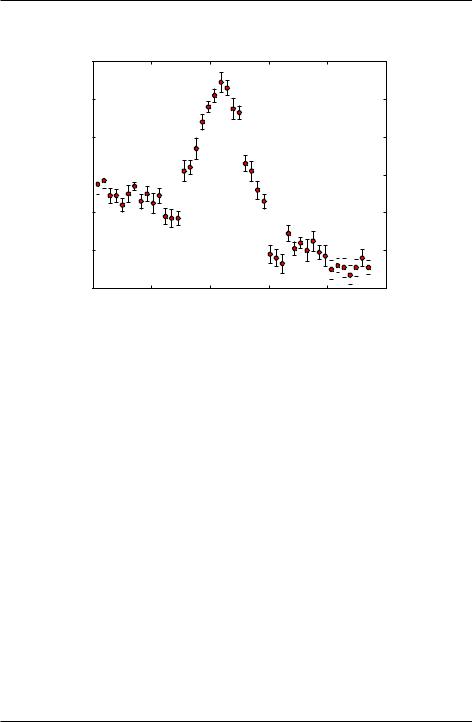
We demonstrate the use of curve_fit to fit the data plotted in the figure below:

We model the data with the fitting function that consists of a quadratic polynomial background with a Gaussian peak:

A(f) = a + bf + cf2 + P e 12 [(f fp)=fw]2 :

Lines 7 and 8 define the fitting functions. Note that the independent variable f is the first argument, which is followed by the six fitting parameters a, b, c, P , fp, and fw.

To fit the data with A(f), we need good estimates of the fitting parameters. Setting f = 0, we see that a 60. An estimate of the slope of the baseline gives b 60=20 = 3. The curvature in the baseline is small so we take c 0. The amplitude of the peak above the baseline is P 80. The peak is centered at fp 11, while width of peak is about fw 2. We use these estimates to set the initial guesses of the fitting parameters in lines 14 and 15 in the code below.

Introduction to Python for Science, Release 0.9.23

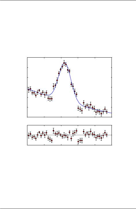
The function that performs the Levenverg-Marquardt algorithm, scipy.optimize.curve_fit, is called in lines 19-20 with the output set equal to the one and two-dimensional arrays nlfit and nlpcov, respectively. The array nlfit, which gives the optimal values of the fitting parameters, is unpacked in line 23. The square root of the diagonal of the twodimensional array nlpcov, which gives the estimates of the uncertainties in the fitting parameters, is unpacked in lines 26-27 using a list comprehension.

The rest of the code plots the data, the fitting function using the optimal values of the fitting parameters found by scipy.optimize.curve_fit, and the values of the fitting parameters and their uncertainties.

1import numpy as np

2import matplotlib.pyplot as plt

3 import matplotlib.gridspec as gridspec # for unequal plot boxes

4import scipy.optimize

5

6# define fitting function

7def GaussPolyBase(f, a, b, c, P, fp, fw):

8return a + b*f + c*f*f + P*np.exp(-0.5*((f-fp)/fw)**2)

9

10# read in spectrum from data file

11# f=frequency, s=signal, ds=s uncertainty

12f, s, ds = np.loadtxt("Spectrum.txt", skiprows=4, unpack=True)

13

Introduction to Python for Science, Release 0.9.23

14# initial guesses for fitting parameters

15a0, b0, c0 = 60., -3., 0.

16P0, fp0, fw0 = 80., 11., 2.

17

18# fit data using SciPy’s Levenberg-Marquart method

19nlfit, nlpcov = scipy.optimize.curve_fit(GaussPolyBase,

22# unpack fitting parameters

23a, b, c, P, fp, fw = nlfit

24# unpack uncertainties in fitting parameters from diagonal

25# of covariance matrix

26da, db, dc, dP, dfp, dfw = \

29# create fitting function from fitted parameters

30f_fit = np.linspace(0.0, 25., 128)

31s_fit = GaussPolyBase(f_fit, a, b, c, P, fp, fw)

32

33# Calculate residuals and reduced chi squared

34resids = s - GaussPolyBase(f, a, b, c, P, fp, fw)

35redchisqr = ((resids/ds)**2).sum()/float(f.size-6)

36

37# Create figure window to plot data

38fig = plt.figure(1, figsize=(8,8))

39gs = gridspec.GridSpec(2, 1, height_ratios=[6, 2])

40

41# Top plot: data and fit

42ax1 = fig.add_subplot(gs[0])

43ax1.plot(f_fit, s_fit)

44ax1.errorbar(f, s, yerr=ds, fmt=’or’, ecolor=’black’)

45ax1.set_xlabel(’frequency (THz)’)

46ax1.set_ylabel(’absorption (arb units)’)

47ax1.text(0.7, 0.95, ’a = {0:0.1f}$\pm${1:0.1f}’

48.format(a, da), transform = ax1.transAxes)

49ax1.text(0.7, 0.90, ’b = {0:0.2f}$\pm${1:0.2f}’

50.format(b, db), transform = ax1.transAxes)

51ax1.text(0.7, 0.85, ’c = {0:0.2f}$\pm${1:0.2f}’

52.format(c, dc), transform = ax1.transAxes)

53ax1.text(0.7, 0.80, ’P = {0:0.1f}$\pm${1:0.1f}’

54.format(P, dP), transform = ax1.transAxes)

55ax1.text(0.7, 0.75, ’fp = {0:0.1f}$\pm${1:0.1f}’

56.format(fp, dfp), transform = ax1.transAxes)

57ax1.text(0.7, 0.70, ’fw = {0:0.1f}$\pm${1:0.1f}’

58.format(fw, dfw), transform = ax1.transAxes)

Introduction to Python for Science, Release 0.9.23

59ax1.text(0.7, 0.60, ’$\chi_r^2$ = {0:0.2f}’

60.format(redchisqr),transform = ax1.transAxes)

61ax1.set_title(’$s(f) = a+bf+cf^2+P\,e^{-(f-f_p)^2/2f_w^2}$’)

62

63# Bottom plot: residuals

64ax2 = fig.add_subplot(gs[1])

65ax2.errorbar(f, resids, yerr = ds, ecolor="black", fmt="ro")

66ax2.axhline(color="gray", zorder=-1)

67ax2.set_xlabel(’frequency (THz)’)

68ax2.set_ylabel(’residuals’)

69ax2.set_ylim(-20, 20)

70ax2.set_yticks((-20, 0, 20))

71

72plt.show()

The above code also plots the difference between the data and fit, known as the residuals in the subplot below the plot of the data and fit. Plotting the residuals in this way gives a graphical representation of the goodness of the fit. To the extent that the residuals vary randomly about zero and do not show any overall upward or downward curvature, or any long wavelength oscillations, the fit would seem to be a good fit.

Finally, we note that we have used the MatPlotLib package gridspec to create the two subplots with different heights. The gridspec are made in lines 3 (where the package is imported), 36 (where 2 rows and 1 column are specified with relative heights of 6 to 2), 39 (where the first gs[0] height is specified), and 54 (where the second gs[1] height is specified). More details about the gridspec package can be found at the MatPlotLib web site.

Introduction to Python for Science, Release 0.9.23

Figure 8.2: Fit to Gaussian with quadratic polynomial background.