Добавил:

fench Опубликованный материал нарушает ваши авторские права? Сообщите нам.

Вуз:

Сумский государственный университет

Предмет:

Биомеханика

Файл:

Intermediate Probability Theory for Biomedical Engineers - JohnD. Enderle

.pdf

Скачиваний:

Добавлен:

10.08.2013

Размер:

966.8 Кб

Скачать

☆

<<< < Предыдущая 1 2 3 4 5 6 7 89 / 129 10 11 12 > Следующая >>>

BIVARIATE RANDOM VARIABLES 73

Solution. (a) We ﬁnd

P (Ac ) = P (x = y) = px,y (1, 1) + px,y (3, 3) = 14 ;

hence, P (A) = 1 − P (Ac ) = 3/4. Let Dx,y denote the support set for the PMF px,y . Then

		px,y (α, β)	, (α, β) Dx,y ∩ {α = β}
px,y\| A(α, β \| A) =		P (A)	, (α, β) Dx,y ∩ {α = β}
	0,				otherwise.
The result is shown in graphical form in Fig. 4.13.
(b) We have
	py\|x (β \| 1) =			px,y (1, β)	,
	py\|x (β \| 1) =			px (1)	,

and

3 px (1) = Px,y (1, β) = Px,y (1, −1) + Px,y (1, 1) = 8 .

Consequently,

		1/3,		β = 1
px\|y (β \| 1) = 2/3,				β = −1
		0,		otherwise.
		b
		1
		6
	2
1	1			1
6	1			6
6				6
1 6
-1		1	2	3	a
	-1	1
	-1	3
		3

FIGURE 4.13: Conditional PMF for Example 4.5.1a.

74INTERMEDIATE PROBABILITY THEORY FOR BIOMEDICAL ENGINEERS

(c)The support set for px,y is {(−1, 0), (−1, 1)}, and we ﬁnd easily that P (B) = 1/4. Then

0.5, (α, β) = (−1, 0)

px,y|B (α, β | B) = 0.5, (α, β) = (−1, 1)

otherwise.

Thus

px|B

(α

| B

)

α = −1

otherwise,

and

0.5,

β = 0

py|B (β | B) = 0.5,

β = 1

otherwise.

We conclude that x and y are conditionally independent, given B.

Example 4.5.2. Random variables x and y have joint PDF

fx,y

(α, β)

0.25α(1 + 3β2), 0 < α < 2, 0 < β < 1

otherwise.

Find (a) P (0 < x < 1|y = 0.5) and (b) fx,y| A(α, β | A), where event A = {x + y ≤ 1}.

Solution. (a) First we ﬁnd

α 7

fy (0.5) =

d α =

Then for 0 < α < 2,

fx|y (α | 0.5) =

0.25α7/4

7/8

and

P (0 < x < 1|y = 0.5) =

0 α

d α =

(b) First, we ﬁnd

P (A) =

α+β≤1

fx,y (α, β)d αdβ;

BIVARIATE RANDOM VARIABLES

substituting,

1−β

P (A) =

(1 + 3β2) d

αdβ =

240

The support region for the PDF fx,y

R = {(α, β) : 0 < α < 2, 0 < β < 1}.

Let B = R ∩ {α + β ≤ 1}. For all (α, β) B, we have

fx,y (α, β)

fx,y| A(α, β | A) =

α(1 + 3β2),

P (A)

and fx,y| A(α, β | A) = 0, otherwise. We note that

B = {(α, β) : 0 < α ≤ 1 − β < 1}.

Example 4.5.3. Random variables x and y have joint PDF

fx,y

(α, β)

6α, 0 < α < 1 − β < 1

otherwise.

Determine whether or not x and y are conditionally independent, given A = {ζ S : x ≥ y}.

Solution. The support region for fx,y is

R = {(α, β) : 0 < α < 1 − β < 1}; the support region for fx,y| A is thus

B = {(α, β) : 0 < α < 1 − β < 1, α ≥ β} = {0 < β ≤ α < 1 − β < 1}.

The support regions are illustrated in Fig. 4.14.

1	b			1
1				1
0.5				0.5
	R
0	0.5	1	a	0

b
B
0.5	1	a

FIGURE 4.14: Support regions for Example 4.5.3.

76 INTERMEDIATE PROBABILITY THEORY FOR BIOMEDICAL ENGINEERS

		b
3	1		1		1

	8		8		8
	8		8		8
2	1		1

	8		4
	8		4
1			1		1

			8		8
			8		8
0

						a
	1		2	3		a

FIGURE 4.15: PMF for Drill Problem 4.5.1.

For (α, β) B,

fx,y| A(α, β | A) =

fx,y (α, β)

6α

P (A)

The conditional marginal densities are found by integrating

fx,y| A:

For 0 < β < 0.5,

1−β

3(1 − 2β)

fy| A(

| A) =

P (A)

For 0 < α < 0.5,

6α2

fx| A(α | A) =

6α dβ =

P (A)

For 0.5 < α < 1,

1−α

6α(1 − α)

fx| A(

| A) =

P (A)

We conclude that since P (A) is a constant, the RVs x and y are not conditionally independent, given A.

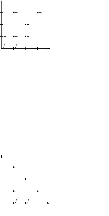
Drill Problem 4.5.1. Random variables x and y have joint PMF shown in Fig. 4.15. Find (a) px (1), (b) py (2), (c ) px|y (1 | 2), (d ) py|x (3 | 1).

Answers: 1/2, 1/4, 3/8, 1/3.

BIVARIATE RANDOM VARIABLES 77

3	1			1
3	8			8
	8			8
2			1
2			8
			8
1	1		1
1	8		8
8	8		8
1 8	1 8			a
0	1	2	3	a
	1	2	3

FIGURE 4.16: PMF for Drill Problem 4.5.2.

Drill Problem 4.5.2. Random variables x and y have joint PMF shown in Fig. 4.16. Event A = {ζ S : x + y ≤ 1}. Find (a) P (A), (b) px,y| A(1, 1 | A), (c ) px| A (1 | A), and (d) py| A(1 | A).

Answers: 0, 3/8, 1/3, 1/3.

Drill Problem 4.5.3. Random variables x and y have joint PMF shown in Fig. 4.17. Determine if random variables x and y are: (a) independent, (b) independent, given {y ≤ 1}.

Answers: No, No.

Drill Problem 4.5.4. The joint PDF for the RVs x and y is

		2	α2β, 0 < α < 3, 0 < β < 1
fx,y (α, β) = 9			α2β, 0 < α < 3, 0 < β < 1
fx,y (α, β) = 9			0,				otherwise.
			0,				otherwise.
3	b		1
	b


			8
			8
2					1

					4
					4
1			1					1

			8					8
			8					8
				1 4		1 8
				1 4		1 8
0									a
0			1		2		3		a
			1		2		3

FIGURE 4.17: PMF for Drill Problem 4.5.3.

78 INTERMEDIATE PROBABILITY THEORY FOR BIOMEDICAL ENGINEERS

Find: (a) fx|y (1 | 0.5), (b) fy|x (0.5 | 1), (c )P (x ≤ 1, y ≤ 0.5 | x + y ≤ 1), and (d) P (x ≤ 1 | x + y ≤ 1).

Answers: 1/9, 1, 1, 13/16.
Drill Problem 4.5.5.			The joint PDF for the RVs x and y is
				fx,y (α, β) = e −α−β u(α)u(β).
Find: (a) fx\|y (1 \| 1), (b)Fx\|y (1 \| 1), (c )P (x ≥ 5 \| x ≥ 1), and (d) P (x ≤ 0.5 \| x + y ≤ 1).
Answers: 1	−	e −1, e −1	, e −4,	1 − e −0.5 − 0.5e −1			.
Answers: 1		e −1, e −1	, e −4,				.
				1 − 2e −1
Drill Problem 4.5.6.			The joint PDF for the RVs x and y is
					2β	, 0 < β < √				< 1
					2β				α
									α
			fx,y (α, β) = α					otherwise.
				0,				otherwise.
Find: (a)	P (y ≤ 0.25 \| x = 0.25), (b)P (y = 0.25 \| x = 0.25), (c )P (x ≤ 0.25 \| x ≤ 0.5), and
(d) P (x ≤ 0.25 \| x + y ≤ 1).

Answers: 0, 1/2, 1/4, 0.46695.

Drill Problem 4.5.7. The joint PDF for the RVs x and y is

fx,y (α, β) =	4αβ,	0 < α < 1, 0 < β < 1
fx,y (α, β) =	0,	otherwise.

Determine whether or not x and y are (a) independent, (b) independent, given A = {x + y ≥ 1}.

Answers: No, Yes.

4.6CONDITIONAL EXPECTATION

Conditional expectation is completely analogous to ordinary expectation, with the unconditional CDF replaced with the conditional version. In particular, the conditional expectation of g (x, y), given event A, is deﬁned as

∞ ∞

E(g (x, y) \| A) =	g (α, β) d Fx,y\|A(α, β \| A) .	(4.77)
	−∞ −∞

When the conditioning event A has zero probability, as when A = {x = 0} for continuous RVs, the conditional CDF, PMF, and PDF deﬁnitions of the previous sections are used.

BIVARIATE RANDOM VARIABLES 79

Deﬁnition 4.6.1. The conditional expectation of g (x, y), given y = β, is deﬁned by

∞

E(g (x, y) \| y = β) = g (α, β) d Fx\|y (α \| β).		(4.78)
−∞
In particular, the conditional mean of x, given y = β, is
∞	∞
E(x \| y = β) = α d Fx\|y (α \| β) =	α fx\|y (α \| β) d α .	(4.79)
−∞	−∞

It is important to note that if the given value of y(β) is a constant, then E(x | y = β) is also a constant. In general, E(x | y = β) is a function of β. Once this function is obtained, one may substitute β = y(ζ ) and treat the result as a random variable; we denote this result as simply E(x | y). It is also important to note that conditional expectation, as ordinary expectation, is a linear operation.

Deﬁnition 4.6.2. The conditional mean of x, given y = β, is deﬁned by
	ηx\|y=β = E(x\|y = β),								(4.80)
note that the RV ηx\|y = E(x \| y). The conditional variance of x, given y = β, is deﬁned by
σx2\|y=β = E((x − ηx\|y )2\|y = β).									(4.81)
The RV σx2\|y = E((x − ηx\|y )2\|y).
Example 4.6.1. Random variable y has PMF
			0.25,				α = 1
py	(α)	=	0.5,				α = 2
py		=	0	.	25	,	α	= 3
			0		25			= 3
				0,			otherwise.
Find the variance of y, given event A = {y odd}.
Solution. We easily ﬁnd P (A) = 0.5 so that
					0.5,		α = 1
py\| A(α \| A) = 0.5,							α = 3
					0,		otherwise.

80 INTERMEDIATE PROBABILITY THEORY FOR BIOMEDICAL ENGINEERS

Then

ηy| A = E(y| A) =

α2 py|a (α| A) = 2

and

E(y2| A) =

α2 py| A(α| A) = 5.

Finally,

σy2| A = E(y2| A) − E2(y| A) = 5 − 4 = 1.

Example 4.6.2. Random variables x and y have joint PDF

fx,y

(α, β)

2, α > 0, 0 < β < 1 − α

otherwise.

Find ηx|y = E(x|y), E(ηx|y ), and E(x).

Solution. We ﬁrst ﬁnd the marginal PDF

∞

1−β

fy (β) =

fx,y (α, β) d α =

2 d α = 2(1 − β),

−∞

for 0 < β < 1. Then for 0 < β < 1,

fx,y (α, β)

, 0 < α < 1 − β

fx|y (

)

1 −

fy (β)

otherwise.

Hence, for 0 < β < 1,

1−β

1 − β

E(x | y = β) =

d α =

1 −

We conclude that

x|y

= E(x | y) =

1 − y

Now,

x|y )

= E

1 − y

1 − β

2(1 −

= E(x)

																								BIVARIATE RANDOM VARIABLES													81
Example 4.6.3.				Find the conditional variance of y, given A = {x ≤ 0.75}, where
Example 4.6.3.
				fx,y (α, β) = 1.5(α2 + β2)(u(α) − u(α − 1))(u(β) − u(β − 1)).
Solution. First, we ﬁnd
										1	0.75													75
																								75
								P (A) =			1.5(α2							+		β2) d αdβ =												,
								P (A) =			1.5(α2							+		β2) d αdβ =							128					,
										0	0
so that
			(α, β			A)			fx,y (α, β)				64			(α2 + β2), 0 < α < 0.75, 0 < β < 1
f	,	y\| A			\|		=		fx,y (α, β)		=
f	,								P (A)
	x								P (A)				25					0,													otherwise.
																		0,													otherwise.
Then for 0 < β < 1,
						fy\| A(β \| A) =					0.75 64				α2						β2 d			9					48							β2.
																		+						α =					+
										0		25						+						α =		25			+				25
Consequently,
											1		9					48											66
													9					48											66
							E(y \| A) =				β						+					β2		d α =										,
							E(y \| A) =				β			25			+		25			β2		d α =				100						,
											0
and
											1		9							48									378
													9							48									378
							E(y2 \| A) =				β2							+					β2	d α =											.
							E(y2 \| A) =				β2		25					+			25		β2	d α =						750					.
											0
Finally,
									σy2\| A = E(y2 \| A) − E2															513
																				(y \| A) =											.
																				(y \| A) =					7500						.
There are many applications of conditional expectation. One important use is to simplify
calculations involving expectation, as by applying the following theorem.
Theorem 4.6.1. Let x and y be jointly distributed RVs. Then
									E(g (x, y)) = E(E(g (x, y) \| y))																				(4.82)
Proof. Note that
									d Fx,y (α, β) = d Fx\|y (α \| β) dFy (β).
									d Fx,y (α, β) = d Fx\|y (α \| β) dFy (β).

82 INTERMEDIATE PROBABILITY THEORY FOR BIOMEDICAL ENGINEERS

Special cases of this are

fx,y (α, β) = fx|y (α | β) fy (β)

and

px,y (α, β) = px|y (α | β) py (β).

We thus have

∞	∞
E(g (x, y)) =	g (α, β) d Fx\|y (α \| β) dFy (β).
−∞	−∞
Hence
	∞
E(g (x, y)) = E(g (x, y) \| y = β) dFy (β),
	−∞
from which the desired result follows.
The conditional mean estimate is one of the most important applications of conditional
expectation.
Theorem 4.6.2. Let x and y be jointly distributed RVs with σx2 < ∞. The function g		which
minimizes E((x − g (y))2) is
	g (y) = E(x \| y).	(4.83)
Proof. We have

E((x − g (y))2 | y) = E((x − ηx|y + ηx|y − g (y))2 | y)

=σx2|y + 2E((x − ηx|y )(ηx|y − g (y))|y) + (ηx|y − g (y))2

=σx2|y + (ηx|y − g (y))2.

The choice g (y) = ηx|y is thus seen to minimize the above expression, applying the (unconditional) expectation operator yields the desired result.

The above result is extremely important: the best minimum mean square estimate of a quantity is the conditional mean of the quantity, given the data to be used in the estimate. In many cases, the conditional mean is very difﬁcult or even impossible to compute. In the important Gaussian case (discussed in a later chapter) the conditional mean turns out to be easy to ﬁnd. In fact, in the Gaussian case, the conditional mean is always a linear function of the given data.

<<< < Предыдущая 1 2 3 4 5 6 7 89 / 129 10 11 12 > Следующая >>>

Соседние файлы в предмете Биомеханика

#
10.08.20133.54 Mб221Environmental Biotechnology - Theory and Application - G. M. Evans & J. C. Furlong.pdf
#
10.08.20139.65 Mб50Genomics and Proteomics Engineering in Medicine and Biology - Metin Akay.pdf
#
10.08.20132.2 Mб54Glossary of Biotechnology Terms - Kimball Nill.pdf
#
10.08.20135.05 Mб74Image and Signal Processing for Networked E-Health Applications - Ilias G. Maglogiannis.pdf
#
10.08.201320.85 Mб93Intermediate Physics for Medicine and Biology - Russell K. Hobbie & Bradley J. Roth.pdf
#
10.08.2013966.8 Кб79Intermediate Probability Theory for Biomedical Engineers - JohnD. Enderle.pdf
#
10.08.201335.92 Mб65Introduction to Biomedical Engineering - John D. Enderle et al.pdf
#
10.08.20131.72 Mб126Introduction to Statistics for Biomedical Engineers - Kristina M. Ropella.pdf
#
10.08.201310.58 Mб106Kluwer - Handbook of Biomedical Image Analysis Vol.1.pdf
#
10.08.201325.84 Mб102Kluwer - Handbook of Biomedical Image Analysis Vol.2.pdf
#
10.08.201316.35 Mб110Kluwer - Handbook of Biomedical Image Analysis Vol.3.pdf