Intermediate Probability Theory for Biomedical Engineers - JohnD. Enderle

Добавил:

fench Опубликованный материал нарушает ваши авторские права? Сообщите нам.

Вуз:

Сумский государственный университет

Предмет:

Биомеханика

Файл:

P (ζ S : x(ζ ) ≤ α, y(ζ ) ≤ β, ζ A)

provided that P (A) = 0.

A = {ζ : y(ζ ) = β}.

In this section, we extend this notion to the conditioning event

.pdf

Скачиваний:

Добавлен:

10.08.2013

Размер:

966.8 Кб

Скачать

☆

<<< < Предыдущая 1 2 3 4 5 6 78 / 128 9 10 11 12 > Следующая >>>

BIVARIATE RANDOM VARIABLES 63

Proof. If either a = 0 or b = 0 then P (xy = 0) = 1 so that E(|xy|) = 0; hence, assume a > 0 and b > 0. Let

g (α) = α p + βq − αβ, p q

for α ≥ 0, β > 0. We have g (0) > 0, g (∞) = ∞, g (1)(α) = α p−1 − β, and g (2)(α0) = ( p − 1)α0p−2 > 0, where α0 satisﬁes g (1)(α0) = 0. Thus, g (α) ≥ g (α0), and α0 = β1/( p−1) = βq / p . Consequently,

α p		βq			α0p	βq
		+		− αβ ≥		+		− α0β = 0.
	p	+	q	− αβ ≥	p	+	q	− α0β = 0.
The desired result follows by letting α = \|x\|/a and β = \|y\|/b.
Corollary 4.3.1. (Schwarz Inequality)
			E2(\|xy\|) ≤ E(\|x\|2)E(\|y\|2).						(4.52)
If y = a x, for some constant a, then
E2(\|xy\|) = \|a\|2 E2(\|x\|2) = E(\|x\|2)E(\|y\|2).
Applying the Schwarz Inequality, we ﬁnd that the covariance between x and y satisﬁes
	σx2,y = E2((x − ηx )(y − ηy )) ≤ σx2σy2.
Hence, the correlation coefﬁcient satisﬁes
				\|ρx,y \| ≤ 1.					(4.53)

If there is a linear relationship between the RVs x and y, then |ρx,y | = 1, as shown in Example 4.3.1.

Theorem 4.3.5. (Minkowski Inequality) Let p be a real constant with p ≥ 1. If x and y are RVs with E(|x|p ) < ∞ and E(|y| p ) < ∞ then

E1/ p (|x + y|p ) ≤ E1/ p (|x|p ) + E1/ p (|y|p ).

(4.54)

Proof. From the triangle inequality (|x + y| ≤ |x| + |y|),

E(|x + y|p ) = E(|x + y||x + y|p−1)

≤ E(|x||x + y|p−1) + E(|y||x + y|p−1),

φx+y (t) = φx (t)φy (t).

64 INTERMEDIATE PROBABILITY THEORY FOR BIOMEDICAL ENGINEERS

which yields the desired result if p = 1. For p > 1, let q = p/( p − 1) and apply the Holder¨ Inequality to obtain

E(|x + y|p ) ≤ E1/ p (|x| p )E1/q (|x + y|p ) + E1/ p (|y|p )E1/q (|x + y|p ),

from which the desired result follows.
Theorem 4.3.6. With αk = E1/ k (\|x\|k ) we have αk+1 ≥ αk for k = 1, 2, . . . .
Proof. Let βi = E(\|x\|i ). From the Schwarz inequality,
βi2 = E2(\|x\|(i−1)/2\|x\|(i+1)/2) ≤ E(\|x\|i−1)E(\|x\|i+1) = βi−1βi+1.
Raising to the ith power and taking the product (noting that β0 = 1)
k		k		k−1	k+1	k−1
βi2i ≤ βii−1βii+1 = βii+1					β jj −1 = βkk−1βkk+1	βi2i .
i=1		i=1		i=0	j =2	i=1
Simplifying, we obtain	βk+1		≤	βk			/	(k(k + 1))
Simplifying, we obtain	k		≤	k+1; the desired inequality follows by raising to the 1				(k(k + 1))
power.

4.3.3Joint Characteristic Function

Deﬁnition 4.3.4. The joint characteristic function for the RVs x and y is deﬁned by

φx,y (t1, t2) = E(e j xt1+ j yt2 ),

(4.55)

where t1 and t2 are real variables, and j 2 = −1.

Note that the marginal characteristic functions φx and φy are easily obtained from the joint characteristic function as φx (t) = φx,y (t, 0) and φy (t) = φx,y (0, t).

Theorem 4.3.7. The joint RVs x and y are independent iff

φx,y (t1, t2) = φx (t1)φy (t2)

(4.56)

for all real t1 and t2.

Theorem 4.3.8. If x and y are independent RVs, then

(4.57)

Theorem 4.3.9. The joint (m,n)th moment of the RVs x and y can be obtained from the joint characteristic function as

E(x	m	y	n	) = (− j )	m+nφ(m,n)	(0	,	0)	.	(4.58)
					x,y

BIVARIATE RANDOM VARIABLES 65

The joint characteristic function φx,y contains all of the information about the joint CDF Fx,y ; the joint CDF itself can be obtained from the joint characteristic function.

Theorem 4.3.10.

If the joint CDF Fx,y is continuous at (a1, a2) and at (b1, b2), with a1 < b1

and a2 < b2, then

e − j a2t2 − e − j b2t2

P (a1

x ≤ b1

y ≤ b2) = Tlim

e − j a1t1 − e − j b1t1

x,y (t1

t2) d t1 d t2

j 2

→∞

−T −T

(4.59)

Proof. The proof is a straightforward extension of the corresponding one-dimensional

result.
Corollary 4.3.2. If x and y are jointly continuous RVs with φx,y , then
	1			T	T
fx,y (α, β) = Tlim	1				e − j αt1− jβt2 φx,y (t1, t2) d t1 d t2 .	(4.60)

	π	)	2
→∞ (2		)

−T −T

The above corollary establishes that the joint PDF is 1/(2π )2 times the two-dimensional Fourier transform of the joint characteristic function.

Drill Problem 4.3.1. The joint PDF for RVs x and y is

	2	α2β, 0 < α < 3, 0 < β < 1
fx,y (α, β) = 9
		0,	otherwise.

Find σx,y .

Answer: 0.

Drill Problem 4.3.2. Suppose the RVs x and y have the joint PMF shown in Fig. 4.11. Determine:

(a) E(x), (b)E(y), (c )E(x + y), and (d) σx,y .

Answers: 0.54, 1.6, 3.2, 1.6.

Drill Problem 4.3.3.		Suppose ηx = 5, ηy = 3, σx,y = 18, σx = 3, and σy = 6. Find: (a) E(x2),
(b)E(xy), (c )σ 2	, and (d) σ 2		.
3x		x+y

Answers: 81, 81, 33, 34.

66 INTERMEDIATE PROBABILITY THEORY FOR BIOMEDICAL ENGINEERS

	b
3	1	2
3	6	10
	6	10
2	1	1
2	10	10
	10	10
1	1	2
1	10	10
	10	10

2 10

0	1	2	3	a

FIGURE 4.11: PMF for Drill Problem 4.3.2.

4.4CONVOLUTION

The convolution operation arises in many applications. Convolution describes the basic input/output relationship for a linear, time-invariant system, as well as the distribution function for the sum of two independent RVs.

Theorem 4.4.1. If x and y are independent RVs and z = x + y then

Fz(γ ) =	∞	∞
Fz(γ ) =	Fx (γ − β)d Fy (β) =	Fy (γ − α)d Fx (α).	(4.61)
	−∞	−∞
The above integral operation on the functions Fx and Fy is called a convolution.
Proof. By deﬁnition,
Fz(γ ) = P (z ≤ γ ) =		d Fx,y (α, β).
	α+β≤γ
Since x and y are independent, we have
	∞ γ −β	∞
Fz(γ ) =	d Fx (α) d Fy (β) = Fx (γ − β) d Fy (β).
	−∞ −∞	−∞
Interchanging the order of integration,
	∞ γ −α	∞
Fz(γ ) =	d Fy (β) d Fx (α) = Fy (γ − α) d Fx (α).
	−∞ −∞	−∞

BIVARIATE RANDOM VARIABLES 67

Corollary 4.4.1. Let x and y be independent RVs and let z = x + y.

(i) If x is a continuous RV then z is a continuous RV with PDF

∞

	fz(γ ) =	fx (γ − β) d Fy (β).		(4.62)
		−∞
(ii) If y is a continuous RV then z is a continuous RV with PDF
		∞
	fz(γ ) =	fy (γ − α) d Fx (α).		(4.63)
		−∞
(iii) If x and y are jointly continuous RVs then z is a continuous RV with PDF
	∞		∞
fz(γ ) =	fx (γ − β) fy (β) dβ =		fy (γ − α) fx (α) d α.	(4.64)
	−∞		−∞

(iv) If x and y are both discrete RVs then z is a discrete RV with PMF

pz(γ ) =	px (γ − β) py (β) = py (γ − α) px (α).	(4.65)
β	α

All of these operations are called convolutions.

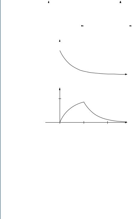
Example 4.4.1. Random variables x and y are independent with fx (α) = 0.5(u(α) − u(α − 2)), and fy (β) = e −β u(β). Find the PDF for z = x + y.

Solution. We will ﬁnd fz using the convolution integral

∞

fz(γ ) = fy (β) fx (γ − β) dβ.

−∞

It is important to note that the integration variable is β and that γ is constant. For each ﬁxed value of γ the above integral is evaluated by ﬁrst multiplying fy (β) times fx (γ − β) and then ﬁnding the area under this product curve. We have

fx (γ − β) = 0.5(u(γ − β) − u(γ − β − 2)).

Plots of fx (α) vs. α and fx (γ − β) vs. β, respectively, are shown in Fig. 4.12(a) and (b). The PDF for y is shown in Fig. 4.12(c). Note that Fig. 4.12(b) is obtained from Fig. 4.12(a) by ﬂipping the latter about the α = 0 axis and relabeling the origin as γ . Now the integration limits for the desired convolution can easily be obtained by superimposing Fig. 4.12(b) onto Fig. 4.12(c)—the value of γ can be read from the β axis.

68 INTERMEDIATE PROBABILITY THEORY FOR BIOMEDICAL ENGINEERS

fx (a)

fx (g−b)

0.5

(g - 2)

(a) fx(a) vs. a.

(b) fx(g - b) vs. b.

fy ( b)

fz (g)

0.5

(d) fz(g) vs. g.

FIGURE 4.12: Plots for Example 4.4.1.

For γ < 0, we have fx (γ − β) fy (β) = 0 for all β; hence, fz(γ ) = 0 for γ < 0. For 0 < γ < 2,

fz(γ ) = 0.5e −β dβ = 0.5(1 − e −γ ).

−∞

For 2 < γ ,

fz(γ ) = 0.5e −β dβ = 0.5e −γ (e 2 − 1).

γ −2

BIVARIATE RANDOM VARIABLES 69

Since the integrand is a bounded function, the resulting fz is continuous; hence, we know that at the boundaries of the above regions, the results must agree. The result is

0,	γ ≤ 0
fz(γ ) = 0.5(1 − e −γ ),	0 ≤ γ ≤ 2
0.5e −γ (e 2 − 1),	2 ≤ γ .

The result is shown in Fig. 12.2(d).

One strong motivation for studying Fourier transforms is the fact that the Fourier transform of a convolution is a product of Fourier transforms. The following theorem justiﬁes this statement.

Theorem 4.4.2. Let Fi be a CDF and

	∞
φi (t) =	e j αt dFi (α),	(4.66)
−∞
for i = 1, 2, 3. The CDF F3 may be expressed as the convolution
∞
F3(γ ) =	F1(γ − β) dF2(β)	(4.67)
−∞

iff φ3(t) = φ1(t)φ2(t) for all real t.

Proof. Suppose F3 is given by the above convolution. Let x CDFs F1 and F2, respectively. Then z = x + y has CDF F3

φ1φ2.

and y be independent RVs with and characteristic function φ3 =

Now suppose that φ3 = φ1φ2. Then there exist independent RVs x and y with characteristic functions φ1 and φ2 and corresponding CDFs F1 and F2. The RV z = x + y then has characteristic function φ3, and CDF F3 given by the above convolution.

It is important to note that φx+y = φx φy is not sufﬁcient to conclude that the RVs x and y are independent. The following example is based on [4, p. 267].

Example 4.4.2. The RVs x and y have joint PDF

fx,y	(α, β)	=	0.25(1 + αβ(α2 − β2)),	\|α\| ≤ 1, \|β\| ≤ 1
fx,y		=	0,	otherwise.

Find: (a) fx and fy , (b)φx and φy , (c )φx+y , (d ) fx+y .

70 INTERMEDIATE PROBABILITY THEORY FOR BIOMEDICAL ENGINEERS

Solution. (a) We have

0.5,

|α| ≤ 1

(α)

αβ(α2

−

β2))

−1

otherwise.

Similarly,

0.5,

|β| ≤ 1

(β)

αβ(α2

−

β2))

−1

otherwise.

(b) From (a) we have

sin t

φx (t) =

φy (t) =

e j αt d α =

−1

e j αt e jβt d α dβ + I,

φx+y (t) =

−1 −1

where

αβ(α2 − β2)e j αt e jβt d α dβ.

I =

−1 −1

Interchanging α and β and the order of integration, we obtain

I =

βα(β2 − α2)e jβt e j αt d α dβ = −I.

−1 −1

Hence, I = 0 and

φx+y (t) =

sin t

so that φx+y = φx φy even though x and y are not independent. (d) Since φx+y = φx φy we have

∞

fx+y (γ ) = fx (γ − β) fy (β) dβ.

−∞

BIVARIATE RANDOM VARIABLES

For −1 < γ + 1 < 1 we ﬁnd

γ +1

γ + 2

fx+y (

) =

4 d

−1

For −1 < γ − 1 < 1 we ﬁnd

2 − γ

fx+y (

) =

4 d

γ −1

Hence

fx+y

(γ )

(2 − |γ |)/4,

|γ | ≤ 2

otherwise.

Drill Problem 4.4.1. Random variables x and y have joint PDF

fx,y (α, β) =

4αβ,

0 < α < 1, 0 < β < 1

otherwise.

Random variable z = x + y. Using convolution, determine: (a) fz(−0.5), (b) fz(0.5), (c ) fz(1.5), and (d) fz(2.5).

Answers: 1/12, 0, 13/12, 0.

4.5CONDITIONAL PROBABILITY

We previously deﬁned the conditional CDF for the RV x, given event A, as

Fx\| A(	α	\| A) =	P (ζ S : x(ζ ) ≤ α, ζ A)	,	(4.68)
			P (A)

provided that P (A) = 0. The extension of this concept to bivariate random variables is immediate:

Clearly, when the RV y is continuous, P (y = β) = 0, so that some kind of limiting operation is needed.

72 INTERMEDIATE PROBABILITY THEORY FOR BIOMEDICAL ENGINEERS

Deﬁnition 4.5.1. The conditional CDF for x, given y = β, is
Fx\|y (	α	\|	β	lim	Fx,y (α, β) − Fx,y (α, β − h)	,	(4.70)
					Fy (β) − Fy (β − h)
				) = h→0

where the limit is through positive values of h. It is convenient to extend the deﬁnition so that Fx|y (α | β) is a legitimate CDF (as a function of α) for any ﬁxed value of β.

Theorem 4.5.1. Let x and y be jointly distributed RVs.

If x and y are both discrete RVs then the conditional PMF for x, given y = β, is

px\|y (α \| β) =		px,y (α, β)			,
px\|y (α \| β) =			py (β)		,
for py (β) = 0.
If y is a continuous RV then
Fx\|y (α \| β) =	1		∂ Fx,y (α, β)
						,
	fy (β)			∂β		,

for fy (β) = 0.

If x and y are both continuous RVs then the conditional PDF for x, given y = β is

fx\|y (α \| β) =	fx,y (α, β)	,
fx\|y (α \| β) =	fy (β)	,
for fy (β) = 0.

(4.71)

(4.72)

(4.73)

Proof. The desired results are a direct consequence of the deﬁnitions of CDF, PMF, and

PDF.
Theorem 4.5.2. Let x and y be independent RVs. Then for all real α,
Fx\|y (α \| β) = Fx (α).	(4.74)
If x and y are discrete independent RVs then for all real α,
px\|y (α \| β) = px (α).	(4.75)
If x and y are continuous independent RVs then for all real α,
fx\|y (α \| β) = fx (α).	(4.76)

Example 4.5.1. Random variables x and y have the joint PMF shown in Fig. 4.5. (a) Find the conditional PMF px,y| A(α, β | A), if A = {ζ S : x(ζ ) = y(ζ )}. (b) Find the PMF py|x (β | 1).

<<< < Предыдущая 1 2 3 4 5 6 78 / 128 9 10 11 12 > Следующая >>>

Соседние файлы в предмете Биомеханика

#
10.08.20133.54 Mб221Environmental Biotechnology - Theory and Application - G. M. Evans & J. C. Furlong.pdf
#
10.08.20139.65 Mб50Genomics and Proteomics Engineering in Medicine and Biology - Metin Akay.pdf
#
10.08.20132.2 Mб54Glossary of Biotechnology Terms - Kimball Nill.pdf
#
10.08.20135.05 Mб74Image and Signal Processing for Networked E-Health Applications - Ilias G. Maglogiannis.pdf
#
10.08.201320.85 Mб93Intermediate Physics for Medicine and Biology - Russell K. Hobbie & Bradley J. Roth.pdf
#
10.08.2013966.8 Кб79Intermediate Probability Theory for Biomedical Engineers - JohnD. Enderle.pdf
#
10.08.201335.92 Mб65Introduction to Biomedical Engineering - John D. Enderle et al.pdf
#
10.08.20131.72 Mб126Introduction to Statistics for Biomedical Engineers - Kristina M. Ropella.pdf
#
10.08.201310.58 Mб106Kluwer - Handbook of Biomedical Image Analysis Vol.1.pdf
#
10.08.201325.84 Mб102Kluwer - Handbook of Biomedical Image Analysis Vol.2.pdf
#
10.08.201316.35 Mб110Kluwer - Handbook of Biomedical Image Analysis Vol.3.pdf