

Basic Probability Theory for Biomedical Engineers - JohnD. Enderle
.pdfINTRODUCTION 11
The sets A1, A2, . . . , An are collectively exhaustive if
n
S = A1 A2 · · · An = Ai .
i=1
Example 1.1.4. Let S={(x, y) : x ≥ 0, y ≥ 0}, A={(x, y) : x + y < 1}, B = {(x, y) : x < y}, and C = {(x, y) : xy > 1/4}. Are the sets A, B, and C mutually exclusive, collectively exhaustive, and/or a partition of S?
Solution. Since A ∩ C = , the sets A and C are mutually exclusive; however, A ∩ B = and B ∩ C = , so A and B, and B and C are not mutually exclusive. Since A B C = S, the events are not collectively exhaustive. The events A, B, and C are not a partition of S since they are not mutually exclusive and collectively exhaustive.
Definition 1.1.4. The Cartesian product of sets A and B is a set of ordered pairs of elements of A and the elements of B :
A × B = {ζ = (ζ1, ζ2) : ζ1 A, ζ2 B}. |
(1.31) |
The Cartesian product of sets A1, A2, . . . , An is a set of n-tuples (an ordered list of n elements) of elements of A1, A2, . . . , An :
A1 × A2 × · · · × An = {ζ = (ζ1, ζ2, . . . ζn) : ζ1 A1, ζ2 A2, . . . , ζn An}. |
(1.32) |
||
An important example of a Cartesian product is the usual n-dimensional real Euclidean space: |
|
||
Rn = R × R × · · · × R . |
(1.33) |
||
|
|
|
|
|
n terms |
|
|
1.1.2 Notation
We briefly present a collection of some frequently used (and confused) notation. Some special sets of real numbers will often be encountered:
(a, b) = {x : a < x < b},
(a, b] = {x : a < x ≤ b},
[a, b) = {x : a ≤ x < b},
and
[a, b] = {x : a ≤ x ≤ b}.

12 BASIC PROBABILITY THEORY FOR BIOMEDICAL ENGINEERS
Note that if a > b, then (a, b) = (a, b] = [a, b) = [a, b] = . If a = b, then (a, b) = (a, b] = [a, b) = and [a, b] = a. The notation (a, b) is also used to denote an ordered pair—we depend on the context to determine whether (a, b) represents an open interval of real numbers or an ordered pair.
We will often encounter unions and intersections of a collection of indexed sets. The shorthand notations
n |
Am Am+1 · · · An, |
if n ≥ m |
|
|
Ai = |
(1.34) |
|||
, |
if n < m, |
|||
i=m |
|
|
|
|
and |
|
|
|
|
n |
Am ∩ Am+1 ∩ · · · ∩ An, |
if n ≥ m |
|
|
Ai = |
(1.35) |
|||
S, |
if n < m |
|||
i=m |
|
|
|
are useful for reducing the length of expressions. These conventions are similar to the notation used to express sums and products of real numbers:
n |
xm + xm+1 + · · · + xn, |
if n ≥ m |
|
|
xi = |
(1.36) |
|||
0, |
if n < m, |
|||
i=m |
|
|
|
|
and |
|
|
|
|
n |
xm × xm+1 + · · · + xn, |
if n ≥ m |
|
|
xi = |
(1.37) |
|||
1, |
if n < m. |
|||
i=m |
|
|
|
As with integration, a change of variable is often helpful in solving problems and proving theorems. Consider, for example, using the change of summation index j = n − i to obtain
|
n |
n−1 |
|
xi = |
xn− j . |
|
i=1 |
j =0 |
A corresponding change of integration variable λ = t − τ yields |
||
t |
0 |
t |
|
f (τ )d τ = − f (t − λ)d λ = f (t − λ)d λ . |
|
0 |
t |
0 |
Note that |
|
|
|
3 |
1 |
|
i = 6 = − i = 0, |
|
i=1 |
i=3 |

INTRODUCTION 13
 u(t)
u(t)
1
0 |
t |
FIGURE 1.3: Unit-step function
whereas
3 |
1 |
xdx = 4 = − |
xdx . |
1 |
3 |
In addition to the usual trigonometric functions sin(·), cos(·), and exponential function exp(x) = e x , we will make use of the unit step function u(t) defined as
( |
) |
= |
1, |
if t ≥ 0 |
(1.38) |
u t |
|
0, |
if t < 0. |
In particular, we define u(0) = 1, which proves to be convenient for our discussions of distribution functions in Chapter 2. The unit step function is illustrated in Fig. 1.3.
Drill Problem 1.1.1. Define the sets S = {1, 2, . . . , 9}, A = {1, 2, 3, 4}, B = {4, 5, 8}, and C = {3, 4, 7, 8}. Determine the sets: (a) (A ∩ B)c , (b) (A B C)c , (c ) (A ∩ B) (A ∩ Bc ) (Ac ∩ B), (d ) A (Ac ∩ B) ((A (Ac ∩ B))c ∩ C).
Answers: {1, 2, 3, 4, 5, 7, 8}; {6, 9}; {1, 2, 3, 5, 6, 7, 8, 9}; {1, 2, 3, 4, 5, 8}.
Drill Problem 1.1.2. Using the properties of set operations (not Venn diagrams), determine the validity of the following relationships for arbitrary sets A, B, C, and D : (a) B (Bc ∩ A) = A B, (b) (A ∩ B) (A ∩ Bc ) (Ac ∩ B) = A, (c ) C ∩ (A ((Ac Bc )c ∩ D)) =
A ∩ C, (d ) A (Ac Bc )c = A.
Answers: True, True, True, False.
1.2THE SAMPLE SPACE
An experiment is a model of a random phenomenon, an abstraction which ignores many of the dynamic relationships of the actual random phenomenon. We seek to capture only the prominent features of the real world problem with our experiment so that needless details do not obscure our analysis. Consider our model of resistance, v(t) = Ri(t). One can utilize more accurate models of resistance that will improve the accuracy of our real world analysis, but the

14 BASIC PROBABILITY THEORY FOR BIOMEDICAL ENGINEERS
cost is far too great to sacrifice the simplicity of v(t) = Ri(t) for our work with circuit analysis problems.
Now, we will associate the universal set S with the set of outcomes of an experiment describing a random phenomenon. Specifically, the sample space, or outcome space, is the finest grain, mutually exclusive, and collectively exhaustive listing of all possible outcomes for the experiment. Tossing a fair die is an example of an experiment. In performing this experiment, the outcome is the number on the upturned face of the die, and thus the sample space is S = {1, 2, 3, 4, 5, 6}. Notice that we could have included the distance of the toss, the number of rolls, and other details in addition to the number on the upturned face of the die for the experiment, but unless our analysis specifically called for these details, it would be unreasonable to include them.
A sample space is classified as being discrete if it contains a countable number of objects. A set is countable if the elements can be placed in one-to-one correspondence with the positive integers. The set of integers S = {1, 2, 3, 4, 5, 6} from the die toss experiment is an example of a discrete sample space, as is the set of all integers. In contrast, the set of all real numbers between 0 and 1 is an example of an uncountable sample space. For now, we shall be content to deal with discrete outcome spaces. We will later find that probability theory is concerned with another discrete space, called the event space, which is a countable collection of subsets of the outcome space—whether or not the outcome space itself is discrete.
1.2.1Tree Diagrams
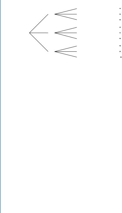
Many experiments consist of a sequence of simpler “subexperiments” as, for example, the sequential tossing of a coin and the sequential drawing of cards from a deck. A tree diagram is a useful graphical representation of a sequence of experiments—particularly when each subexperiment has a small number of possible outcomes.
Example 1.2.1. A coin is tossed twice. Illustrate the sample space with a tree diagram.
Solution. Let Hi denote the outcome of a head on the ith toss and Ti denote the outcome of a tail on the ith toss of the coin. The tree diagram illustrating the sample space for this sequence of two coin tosses is shown in Fig. 1.4. We draw the tree diagram as a combined experiment, in a left to right path from the origin, consisting of the first coin toss (with each of its outcomes) immediately followed by the second coin toss (with each of its outcomes). Note that the combined experiment is really a sequence of two experiments. Each node represents an outcome of one coin toss and the branches of the tree connect the nodes. The number of branches to the right of each node corresponds to the number of outcomes for the next coin toss (or experiment). A sequence of samples connected by branches in a left to right path from the origin to a terminal node represents a sample point for the combined experiment. There

INTRODUCTION 15
Toss 1 |
Toss 2 |
Outcome |
|
H2 |
H1 H2 |
H1 |
|
|
|
T2 |
H1 T2 |
|
H2 |
T1 H2 |
T1 |
|
|
|
T2 |
T1 T2 |
FIGURE 1.4: Tree diagram for Example 1.2.1
is a one-to-one correspondence between the paths in the tree diagram and the sample points in the sample space for the combined experiment. For this example, the outcome space for the combined experiment is
S = {H1 H2, H1T2, T1 H2, T1T2},
consisting of four sample points. |
|
Example 1.2.2. Two balls are selected, one after the other, from an urn that contains nine red, five blue, and two white balls. The first ball is not replaced in the urn before the next ball is chosen. Set up a tree diagram to describe the color composition of the sample space.
Solution. Let Ri , Bi , and Wi , respectively, denote a red, blue, and white ball drawn on the ith draw. Note that R1 denotes the collection of nine outcomes for the first draw resulting in a red ball. We will refer to such a collection of outcomes as an event. The tree diagram shown in Fig. 1.5 is considerably simplified by using only one branch to represent R1, instead of nine. Note that if there were only one white ball (instead of two), the branch terminating with the sequence event W1W2 would be removed from the tree.
Although the tree diagram seems to imply that each outcome is physically followed by the next one, and so on, this need not be the case. A tree diagram can often be used even if the subexperiments are performed at the same time. A sequential drawing of the sample space is only a convenient representation, not necessarily a physical representation.
Example 1.2.3.1 Consider a population with genotypes for the blood disease sickle cell anemia, with the two genotypes denoted by a and b. Assume that b is the code for the anemic trait and that a is without the trait. Individuals can have the genotypes aa, ab and bb. Note that ab and ba are indistinguishable, and that the disease is present only with bb. Construct a tree diagram if both parents are ab.
1This example is based on [14], pages 45–47.
16 BASIC PROBABILITY THEORY FOR BIOMEDICAL ENGINEERS
1st Draw |
2nd Draw |
Event |
Number of outcomes |
||
|
|
R2 |
R1 R2 |
9 |
8 = 72 |
R1 |
B2 |
R1 B2 |
9 |
5 = 45 |
|
|
|
W2 |
R1 W2 |
9 |
2 = 18 |
|
|
R2 |
B1 R2 |
5 |
9 = 45 |
B1 |
B2 |
B1 B2 |
5 |
4 = 20 |
|
|
|
W2 |
B1 W2 |
5 |
2 = 10 |
|
|
R2 |
W1 R2 |
2 |
9 = 18 |
W1 |
B2 |
W1 B2 |
2 |
5 = 10 |
|
|
|
W2 |
W1 W2 |
2 |
1 = 2 |
FIGURE 1.5: Tree diagram for Example 1.2.2
Solution. Background for this problem is given in footnote.2 The tree diagram shown in Fig. 1.6 is formed by first listing the alleles of the first parent and then the alleles of the second parent. Notice only one child out of four will have sickle cell anemia.
2Genetics is the study of the variation within a species, originally based on the work by Mendel in the 19th century. Reproduction is based on transferring genetic information from one generation to the next. Mendel originally called genetic information traits in his work with peas (i.e., stem length characteristic as tall and dwarf, seed shape characteristic as round or wrinkled, etc.). Today we refer to traits as genes, with variations in genes called alleles or genotypes. Each parent stores two genes for each characteristic, and passes only one gene to the progeny. Each gene is equally likely of being passed by the parent to the progeny. Through breeding, Mendel was able to create pure strains of the pea plant, strains that produced only one type of progeny that was identical to the parents (i.e., the two genes were identical). By studying one characteristic at a time, Mendel was able to examine the impact of pure parent traits on the progeny. In the progeny, Mendal discovered that one trait was dominant and the other recessive or hidden. The dominant trait was observed when either parent passed a dominant trait. The recessive trait was observed when both parents passed the recessive trait. Mendel showed that when both parents displayed the dominant trait, offspring could be produced with the recessive trait if both parents contained a dominant and recessive trait, and both passed the recessive trait.
Genetic information is stored in DNA. DNA is a double helix, twisted ladder-like molecule, where pairs of nucleotides appear at each rung joined by a hydrogen bond. The nucleotides are called adenine (A), guanine (G), cytosine (C) and thymine (T). Each nucleotide has a complementary nucleotide that forms a rung; A is always paired with T and G with C, and is directional. Thus if one knows one chain, the other is known. For instance, if one is given AGGTCT, the complement is TCCAGA.
DNA is also described by nucleosomes that are organized into pairs of chromosomes. Chromosomes store all information about the organism’s chemical needs and information about inheritable traits. Humans contain 23 matched pairs of chromosomes. Each chromosome contains thousands of genes that encode instructions for the manufacture of proteins (actually, this process is carried out by messenger RNA)—they are the blueprint for the individual. Each gene has a particular location in a specific chromosome. Slight gene variations exist within a population.
DNA replication occurs during cell division where the double helix is unzipped by an enzyme that breaks the hydrogen bonds that form the ladder rungs, leaving two strands. New double strands are then formed by an elaborate error checking process that binds the appropriate complementary nucleotides. While this process involves

|
|
INTRODUCTION 17 |
Parent 1 |
Parent 2 |
Outcome |
|
a |
aa |
a |
|
|
|
b |
ab |
|
a |
ba |
b |
|
|
|
b |
bb |
FIGURE 1.6: Tree diagram for Example 1.2.3
1.2.2Coordinate System
Another approach to illustrating the outcome space is to use a coordinate system representation. This approach is especially useful when the combined experiment involves a combination of two experiments with numerical outcomes. With this method, each axis lists the outcomes for each subexperiment.
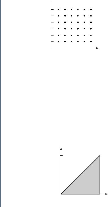
Example 1.2.4. A die is tossed twice. Illustrate the sample space using a coordinate system.
Solution. The coordinate system representation is shown in Fig. 1.7. Note that there are 36 sample points in the experiment; six possible outcomes on the first toss of the die times six possible outcomes on the second toss of the die, each of which is indicated by a point in the coordinate space. Additionally, we distinguish between sample points with regard to order; e.g., (1,2) is different from (2,1).
Example 1.2.5. A real number x is chosen “at random” from the interval [0, 10]. A second real number y is chosen “at random” from the interval [0, x]. Illustrate the sample space using a coordinate system.
Solution. The coordinate system representation is shown in Fig. 1.8. Note that there are an uncountable number of sample points in this experiment.
1.2.3Mathematics of Counting
Although either a tree diagram or a coordinate system enables us to determine the number of outcomes in the sample space, problems immediately arise when the number of outcomes is large. To easily and efficiently solve problems in many probability theory applications, it is
minimal errors (approx. one per billion), errors do happen. The most common error is nucleotide substitution where one is changed for another. For instance, AGGTCT becomes AGCTCT (i.e., the third site goes from G to C). Additional information on this topic is found in [3, 10, 14].
18 BASIC PROBABILITY THEORY FOR BIOMEDICAL ENGINEERS
 2nd Die Toss
6
5
4
3
2
1
0 |
|
|
|
|
|
|
|
|
1 2 3 4 5 6 1st Die Toss |
||||||||
FIGURE 1.7: Coordinate system outcome space for Example 1.2.4
important to know the number of outcomes as well as the number of subsets of outcomes with a specified composition. We now develop some formulas which enable us to count the number of outcomes without the aid of a tree diagram or a coordinate system. These formulas are a part of a branch of mathematics known as combinatorial analysis.
Sequence of Experiments
Suppose a combined experiment is performed in which the first experiment has n1 possible outcomes, followed by a second experiment which has n2 possible outcomes, followed by a third experiment which has n3 possible outcomes, etc. A sequence of k such experiments thus has
n = n1n2 · · · nk |
(1.39) |
y
10
0 |
|
|
x |
|
10 |
||||
|
|
|||
FIGURE 1.8: Coordinate system outcome space for Example 1.2.5

INTRODUCTION 19
Units |
Tens |
Outcome |
|
2 |
27 |
7 |
8 |
87 |
|
9 |
97 |
|
2 |
29 |
9 |
7 |
79 |
|
8 |
89 |
FIGURE 1.9: Tree diagram for Example 1.2.6
possible outcomes. This result allows us to quickly calculate the number of sample points in a sequence of experiments without drawing a tree diagram, although visualizing the tree diagram will lead instantly to the above equation.
Example 1.2.6. How many odd two digit numbers can be formed from the digits 2, 7, 8, and 9, if each digit can be used only once?
Solution. A tree diagram for this sequential drawing of digits is shown in Fig. 1.9. From the origin, there are two ways of selecting a number for the unit’s place (the first experiment). From each of the nodes in the first experiment, there are three ways of selecting a number for the ten’s place (the second experiment). The number of outcomes in the combined experiment is the product of the number of branches for each experiment, or 2 × 3 = 6.
Example 1.2.7. An analog-to-digital (A/D) converter outputs an 8-bit word to represent an input analog voltage in the range −5 to +5 V. Determine the total number of words possible and the maximum sampling (quantization) error.
Solution. Since each bit (or binary digit) in a computer word is either a one or a zero, and there are 8 bits, then the total number of computer words is
n = 28 = 256.
To determine the maximum sampling error, first compute the range of voltage assigned to each computer word which equals
10 V/256 words = 0.0390625 V/word
and then divide by two (i.e., round off to the nearest level), which yields a maximum error of 0.0195312 V/word.

20 BASIC PROBABILITY THEORY FOR BIOMEDICAL ENGINEERS
Sampling With Replacement
Definition 1.2.1. Let Sn = {ζ1, ζ2, . . . , ζn}; i.e ., Sn is a set of n arbitrary objects. A sample of size k with replacement from Sn is an ordered list of k elements:
(ζi1 , ζi2 , . . . , ζik ), where i j {1, 2, . . . , n}, for j = 1, 2, . . . , k.
Theorem 1.2.1. There are nk samples of size k when sampling with replacement from a set of n objects.
Proof. Let Sn be the set of n objects. Each component of the sample can have any of the n values contained in Sn, and there are k components, so that there are nk distinct samples of size k (with replacement) from Sn.
Example 1.2.8. An urn contains ten different balls B1, B2, . . . , B10. If k draws are made from the urn, each time replacing the ball, how many samples are there?
Solution. There are 10k such samples of size k. |
|
Example 1.2.9. How many k-digit base bnumbers are there? |
|
Solution. There are bk different base b numbers. |
|
Permutations
Definition 1.2.2. Let Sn = {ζ1, ζ2, . . . , ζn}; i.e ., Sn is a set of n arbitrary objects. A sample of size k without replacement or permutation from Sn is an ordered list of kelements of Sn :
(ζi1 , ζi2 , . . . , ζik ),
where i j In, j , In,1 = {1, 2, . . . , n}, and In, j = In, j −1 ∩ {i j −1}c , for j = 2, 3, . . . , k.
Theorem 1.2.2. There are
Pn,k = n(n − 1) · · · (n − k + 1)
distinct samples of size k without replacement from a set of n objects. The quantity Pn,k the number of permutations of n things taken k at a time and can be expressed as
n! Pn,k = (n − k)! ,
where n! = n(n − 1)(n − 2) · · · 1, and 0! = 1.
is also called
(1.40)