

Basic Probability Theory for Biomedical Engineers - JohnD. Enderle
.pdfRANDOM VARIABLES 111
|
fx (α ) |
|
|
1 |
|
|
|
0 |
1 |
2 |
α |
|
|||
fx A (α A) |
|
fx B (α B) |
|
|
|
2 |
|
2
|
|
|
|
|
|
|
|
|
|
|
α |
|
|
|
|
|
|
|
|
|
|
|
|
|
|
|
|
α |
0 |
|
1 |
|
|
|
2 |
|
|
0 |
0.5 |
|
|
|
1.5 |
|
|
|
|
||||||||||
|
|
|
|
|
|
|
|
|
|
|
|
|
|
|
||||||||||||||
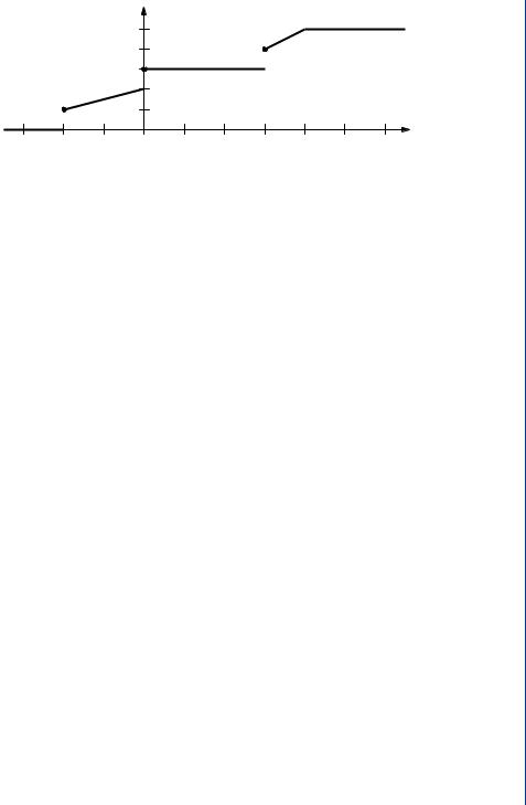
FIGURE 2.10: PDFs for Example 2.5.1 |
|
|
|
|
|
|
|
|
|
|
|
|
|
|
|
|
|
|
|
|||||||||
Consequently, |
|
|
|
|
|
|
|
|
|
|
|
|
|
|
|
|
|
|
|
|
|
|
|
|
|
|
||
|
|
|
|
|
|
|
|
d F |
(α |
B) |
|
|
4(1 − α), |
0.5 < α < 1 |
||||||||||||||
|
|
|
fx|B ( |
α |
|B) = |
|
x|B |
| |
|
= |
4( |
α |
− 1) |
, |
1 |
< α < |
1 |
. |
5 |
|
||||||||
|
|
|
|
d α |
|
|
||||||||||||||||||||||
|
|
|
|
|
|
|
|
|
|
|
|
|
|
|||||||||||||||
|
|
|
|
|
|
|
|
|
|
|
|
|
|
|
0, |
|
|
|
|
|
otherwise. |
|
|
|
||||
The PDFs fx , fx| A, and fx|B are illustrated in Fig. 2.10. |
|
||
Example 2.5.2. The spread of an infection in a family is described by the following PMF |
|||
P ( Sn+1 = k|Sn and In) = |
Sn |
qnk (1 |
− qn)Sn −k |
k |
|||
where n is the sampling interval, Sn+1 is the number of susceptibles during the next sampling interval and Sn is the number of susceptibles during the current sampling interval, In is the number of infectives during the current sampling interval, p is the probability of adequate contact between a susceptible and any infective during one sampling interval, and qn = (1 − p)In is the probability that a susceptible avoids contact with all infectives. This PMF is called the Reed-Frost model and provides the probability of a certain number of susceptibles at a particular sampling interval given a certain number of susceptibles and infectives during the previous sampling internal [2, 10, 14]. If S0 = 5, I0 = 1 and p = 0.2, find the probability that three additional family members are infected by the third sampling interval.

112 BASIC PROBABILITY THEORY FOR BIOMEDICAL ENGINEERS
Solution. Background for this problem is given in footnote.1 This problem is most easily visualized using a tree diagram, from which we find
P (S3 = 2) = P (S3 = 2|S1 = 2, S2 = 2) P (S2 = 2|S1 = 2) P (S1 = 2)
+P (S3 = 2|S1 = 3, S2 = 2) P (S2 = 2|S1 = 3) P (S1 = 3)
+P (S3 = 2|S1 = 3, S2 = 3) P (S2 = 3|S1 = 3) P (S1 = 3)
+P (S3 = 2|S1 = 4, S2 = 2) P (S2 = 2|S1 = 4) P (S1 = 4)
+P (S3 = 2|S1 = 4, S2 = 3) P (S2 = 3|S1 = 4) P (S1 = 4)
+P (S3 = 2|S1 = 4, S2 = 4) P (S2 = 4|S1 = 4) P (S1 = 4)
+P (S3 = 2|S1 = 5, S2 = 2) P (S2 = 2|S1 = 5) P (S1 = 5)
+P (S3 = 2|S1 = 5, S2 = 3) P (S2 = 3|S1 = 5) P (S1 = 5)
+P (S3 = 2|S1 = 5, S2 = 4) P (S2 = 4|S1 = 5) P (S1 = 5)
+P (S3 = 2|S1 = 5, S2 = 5) P S2 = 5 S1 = 5 P (S1 = 5)
=0.64 × 0.64 × 0.0512
+0.64 × 0.384 × 0.2048
+0.384 × 0.512 × 0.2048
+0.64 × 0.1536 × 0.4096
+0.384 × 0.4096 × 0.4096
+0.1536 × 0.4096 × 0.4096
+0.64 × 0.0512 × 0.32768
+0.384 × 0.2048 × 0.32768
+0.1536 × 0.4096 × 0.32768
+0.0512 × 0.32768 × 0.32768
=0.006710886 + 0.050331648 + 0.040265318 + 0.040265318 + 0.064424509
+0.025769804 + 0.010737418 + 0.025769804 + 0.020615843 + 0.005497558
= 0.290388108 |
|
|
1The history of infectious or communicable disease modeling dates to 1760 when D. Bernoulli studied the population dynamics of smallpox with a mathematical model. Little work was done until the early 20th century when Hammer and Soper presented mathematical models which described the spread of measles in Glasgow Scotland. In 1928, Kermack and McKendrick (continuous time), and Reed and Frost (discrete time) presented extensions of the work of Hammer and Soper. Since the 1950s, when Abbey and Bailey presented their work, there has been an epidemic in work in this area.
Infections are spread by adequate contact between two populations, those who are susceptible and those who are infected. The Kermack and McKendrick is a continuous deterministic model that describes the spread of an infection in a large population. The Reed and Frost model is a discrete-time probabilistic model that describes the spread of an infection in a small population. A discrete-time deterministic extension of the Reed and Frost model is useful for exploring the spread of an infection in a large population. One reason for utilizing a discrete-time model rather than a continuous-time model is that recorded data is measured at regular intervals. Another reason is that extensions to this model are easily accomplished, such as adding a nonzero latent period with a precisely defined distribution.

RANDOM VARIABLES 113
Theorem2.5.1(TotalProbability). Let { Ai }in=1 be a partition of S with Ai F, i = 1, 2, . . . , n, and let x be a RV defined on the probability space (S, F, P ). Then
Fx (α) = |
n |
|
Fx| Ai (α| Ai )P (Ai ). |
(2.73) |
|
|
i=1 |
|
Here we assume:
1.Uniform mixing.
2.Nonzero latent period (the time elapsed between contact and the actual discharge of the infectious agent).
3.Population is closed and at steady state.
4.Any susceptible individual after contact with an infectious person develops the infection, and is infectious to others only in the following period, after which they are immune (immune individuals, R, no longer transmits the agent, and are either temporarily or permanently immune to the disease).
5.Since the person can be infected at any instant during the time period — the average latent period is 1/2 of the time period, where the length of the time period represents the period of infectivity.
6.Each individual has a fixed probability of coming into adequate contact p with any other specified individual within one time period.
Note that the probability of adequate contact p can be thought of as
p = average number of adequate contacts .
N
With
q = 1 − p,
the probability that a susceptible individual does not come into adequate contact is
q In .
The structure of the Reed-Frost model is shown in the following diagram.
|
( |
) |
|
|
|
Susceptibles |
1 |
− q In |
Infectives |
|
Immunes |
|
|
|
|||
S |
|
|
I |
|
R |
|
|
|
|
|
|
The Reed-Frost model describes the transfer of S susceptibles, I infectives, and R immunes from state to state at sampling interval n + 1. After adequate contact with an infective in a given sampling interval, a susceptible will develop the infection, and be infectious to others only during the subsequent sampling interval, and after which, becomes immune.
Since order does not matter when a susceptible individual becomes infected, the number of combinations that Sn survive taken k at a time is (kSn ). Then the probability that Sn+1 = k follows as
P ( Sn+1 = k|Sn and In ) |
Sn |
qnk (1 − qn )Sn −k for k = 0, · · · , Sn . |
k |

114 BASIC PROBABILITY THEORY FOR BIOMEDICAL ENGINEERS
If the RV x is discrete, then
px (α) = |
n |
|
Px| Ai (α| Ai )P (Ai ). |
(2.74) |
|
|
i=1 |
|
Similarly, if x is a continuous RV then |
|
|
fx (α) = |
n |
|
fx| Ai (α| Ai )P (Ai ). |
(2.75) |
|
|
i=1 |
|
Proof. Let event B = {ζ : x(ζ ) ≤ α}, and define Bi = B ∩ Ai . Then {Bi }in=1 is a partition of B and
n |
n |
Fx (α) = P (B) = |
p(Bi ) = P (B| Ai )P (Ai ) |
i=1 |
i=1 |
from which the desired results follow. |
|
Example 2.5.3. Resistors are obtained from one of two resistor manufacturers. Manufacturer 1 is event A1 and manufacturer 2 is event A2 with probabilities 1/4 and 3/4, respectively. Given the manufacturer, the conditional PDFs for the resistor values are known as
fr | A1 (α| A1) = 0.01(u(α − 900) − u(α − 1000))
and
fr | A2 (α| A2) = 0.01(u(α − 950) − u(α − 1050)).
Find the PDF of the resistance value.
Solution. From the Theorem of Total Probability, we have
fr (α) = fr | A1 (α| A1)P (A1) + fr | A2 (α| A2)P (A2);
hence, |
|
|
|
|
|
|
1/400, |
900 |
< α < 950 |
||
fr (α) = |
1/100, |
950 |
< α < 1000 |
||
3/400, |
1000 < α < 1050 |
||||
|
0, |
|
|
otherwise. |
|
Drill Problem 2.5.1. A discrete RV x has PMF |
|
|
|||
|
1 |
(0.8)α , α = 1, 2, . . . |
|||
px (α) = |
|
|
|||
|
4 |
||||
|
0, |
|
otherwise. |
||

RANDOM VARIABLES 115
Event A = {ζ : 2 < x(ζ ) < 5} and event B = {ζ : x(ζ ) ≥ 3}. Find (a) px| A(3| A), (b) px|B (4|B).
Answers: 0.16, 0.5556.
Drill Problem 2.5.2. The RV x has PDF fx (α) = e −α u(α), event A = {ζ : x(ζ ) > 10}, and event B = {ζ : −2 < x(ζ ) < 5}. Find fx| A and fx|B .
Answers: e −(α−10)u(α − 10), e −α (u(α) − u(α − 5))/(1 − e −5).
2.6SUMMARY
In this chapter, we have introduced the concept of a random variable. A random variable is a mapping which assigns a real number to each outcome in the sample space. Probabilities for events defined in terms of the random variable x may be computed from the CDF (cumulative distribution function) for x, defined by
Fx (α) = P ({ζ S : x(ζ ) ≤ α}). |
(2.76) |
For example, P (a < x(ζ ) ≤ b) = Fx (b) − Fx (a) if b > a, and P (x(ζ ) = a) = Fx (a) − Fx (a−). Any event of practical interest may be expressed in the form
n |
|
|
|
A = |
Ai , |
|
(2.77) |
i=1 |
|
|
|
where Ai = {x : ai < x ≤ bi } or Ai = {ai }, with Ai ∩ A j = for i = j . Then |
|
||
n |
d Fx(α) = |
n |
|
P (x A) = P (x Ai ) = |
d Fx (α). |
(2.78) |
|
i=1 |
A |
i=1 Ai |
|
Consequently, if the CDF is known, no integration is required.
If the CDF Fx is a jump function (piecewise constant), then x is a discrete RV, with PMF
(probability mass function) |
|
|
px (α) = P (x(ζ ) = α) = Fx (α) − Fx (α−), |
(2.79) |
|
and |
|
|
Fx (α) = |
px (α ), |
(2.80) |
|
α (−∞,α]∩Dx |
|
where Dx is the set of points where px (α) = 0.
If the CDF Fx contains no jumps then (for all practical purposes) x is a continuous RV
with PDF (probability density function) |
|
|
|
fx (α) = |
d Fx (α) |
(2.81) |
|
d α |
|
||

116 BASIC PROBABILITY THEORY FOR BIOMEDICAL ENGINEERS
and
α |
|
Fx (α) = fx (α ) d α . |
(2.82) |
−∞ |
|
The RV x is a mixed RV if it is neither discrete nor continuous. The Lebesgue Decomposition Theorem can be applied in this case to separate the CDF into discrete and continuous parts.
The Riemann-Stieltjes integral was defined in order to provide a unified analytical framework for treating any type of RV. The Dirac delta function provides a useful alternative— enabling one to use a Riemann integral and a PDF containing Dirac delta functions in the mixed or discrete RV cases.
The conditional CDF Fx| A(α| A) was defined as
Fx| A( |
α |
| A) = |
P ({ζ S : x(ζ ) ≤ α and ζ A}) |
, |
(2.83) |
|
P (A) |
||||||
|
|
along with corresponding conditional PDF fx| A and conditional PMF px| A.
2.7PROBLEMS
1.Which of the following functions are legitimate CDF’s? Why, or why not?
|
|
|
0, |
α < −1 |
|
|
|
|
|
H1(α) = α2, |α| ≤ 1 |
|
|
|
|
|||||
|
|
|
1, |
1 < α |
|
|
|
|
|
|
|
|
0, |
α < 0 |
|
|
|
|
|
H2(α) = α2/2, 0 ≤ α ≤ 1 |
|
|
|
||||||
|
|
|
1, |
1 < α |
|
|
|
|
|
H3(α) = |
0, |
α < 0 |
|
|
|
||||
sin(α), 0 ≤ α ≤ π/2 |
|
|
|||||||
|
|
|
1, |
π/2 < α |
|
|
|
||
H4 |
(α) |
= |
0, |
|
α |
|
, |
α ≤ −4 |
|
|
1 − exp(−a( |
+ 4)) |
−4 |
< α |
|||||
|
|
|
|
|
|
||||
2.The sample space is S = {a1, a2, a3, a4} with probabilities P ({a1}) = 0.15, P ({a2}) = 0.25, P ({a3}) = 0.4 and P ({a4}) = 0.2. A random variable x is defined by x(a1) = 2,
RANDOM VARIABLES 117
|
|
Fx (α ) |
|
|
|
1 |
|
|
|
|
0.6 |
|
|
|
|
|
0.4 |
|
|
−2 |
0 |
2 |
4 |
α |
FIGURE 2.11: Cumulative distribution function for Problem 2.6
x(a2) = −1, x(a3) = 3, and x(a4) = 0. Determine: (a) px (α), (b) x−1((−∞, α]), (c) x−1([−1, 2]), and (d) Fx (α).
3.Four fair coins are tossed. Let random variable x equal the number of heads tossed. Determine: (a) px (α), (b) x−1((−∞, α]), and (c) Fx (α).
4.The sample space S = {a1, a2, a3, a4, a5} with probabilities P ({a1}) = 0.15, P ({a2}) = 0.2, P ({a3}) = 0.1, P ({a4}) = 0.25, and P ({a5}) = 0.3. Random variable x is defined as x(ai ) = 2i − 1. Find: (a) px (α), (b) x−1((−∞, α]), and (c) Fx (α).
5.Let
( |
) |
= |
2 − 0.5|t − 5|, |
|t − 5| ≤ 4 |
|||
w t |
|
0 |
, |
|t − 5| |
> |
4 |
|
|
|
|
|
|
|||
Let S = {0, 1, . . . , 19} and P (ζ = i) = 0.05 for i S. Let RV x(ζ ) = w(ζ T) for each
ζS, where T = 0.5. Sketch the CDF for the RV x.
6.Random variable x has CDF shown in Fig. 2.11. Event A = {ζ S : x(ζ ) > 0}, event B = {ζ S : x(ζ ) ≥ 0}, and event C(α) = {ζ S : x(ζ ) ≤ α}. Find: (a) P (x = −2),
(b)P (x = −1), (c) P (0 ≤ x < 3), (d) P (−1 < x ≤ 0), (e) P (B| A), (f ) P (A|B). (g) Find and sketch P (C(α)| A) vs. α.
7.Consider a department in which all of its graduate students range in age from 22 to 28. Additionally, it is three times as likely a student’s age is from 22 to 24 as from 25 to 28. Assume equal probabilities within each age group. Let random variable x equal the age of a graduate student in this department. Determine: (a) px (α), (b) Fx (α).
8.A softball team plays eight games in a season. Assume there are no ties, and that the team has an equal probability of winning or losing each game. Let random variable x equal twice the total number of wins in the season. Determine: (a) px (α), (b) Fx (α),
(c)P (4 ≤ x ≤ 12), (d) P (2 < x ≤ 12), (e) P (12 ≤ x ≤ 20), (f ) P (−1 ≤ x ≤ 12).

118BASIC PROBABILITY THEORY FOR BIOMEDICAL ENGINEERS
9.Which of the following functions are legitimate PDFs? Why? If not, could the function be a PDF if multiplied by an appropriate constant? Find the constant.
0.25, |
−2 < α < 0 |
g1(α) = 0.5, |
1 < α < 3 |
0, |
otherwise |
g2(α) = e −a|α|, |
−∞ < α < ∞ |
|α|, |α| < 1
g3(α) = 0, otherwise
g4(α) = |
sin(π α) |
, |
−∞ < α < ∞ |
π α |
10. Which of the following functions are legitimate PDFs? Why, or why not?
g1 |
(α) |
= |
0.75α(2 − α), 0 ≤ α ≤ 2 |
|||
|
0, |
otherwise |
||||
g2 |
(α) |
= |
0.5e −α , 0 ≤ α < ∞ |
|||
|
0, |
otherwise |
||||
|
|
|
|
√ |
|
|
g |
(α) |
= |
2α − 1, |
0 ≤ α ≤ 0.5(1 + 5) |
||
3 |
|
0, |
otherwise |
|||
g4 |
(α) |
= |
0.5(α + 1), −1 ≤ α ≤ 1 |
|||
|
0, |
otherwise |
||||
11.For the following PDFs, find β, find and sketch the CDF, and then find P (1 ≤ x < 2):
(a)fx (α) = βα2e −3α u(α), (b) fx (α) = β/(1 + α2), (c)
fx |
(α) |
= |
β sin(α), |
0 ≤ α ≤ π/2 |
|
0, |
otherwise |
12. Can a function be both a PDF and CDF? Why or why not?

RANDOM VARIABLES 119
13.The time (in years) before failure, t, for a certain television set is a random variable, with
ft (t0) = 15 e −t0/5u(t0).
Determine: (a) Ft (t0); (b) the probability that the TV set will fail during the first year;
(c) the probability that the TV fails after the 15th year; (d) P (1 < t < 5).
14.The PDF for the time before failure for a piece of equipment is
ft (t0) = βt0 exp(−t0/10)u(t0).
Determine: (a) β; (b) Ft (t0); (c) P (t < 10); (d) P (2 ≤ t < 10). 15. Given CDF
Fx (α) = |
1 |
(α + 1)(u(α + 1) |
− u(α − 2)) |
+ |
1 |
+ |
α |
4 |
2 |
8 |
×(u(α − 2) − u(α − 4)) + u(α − 4),
Determine: (a) fx (α), (b) P (1/4 ≤ x < 3).
16. Given
βα1/2, fx (α) = 0,
Determine: (a) β, (b) Fx (α), (c) P (x ≤ 3/4). 17. Find the CDF for the following PDF
0 < α < 1 otherwise.
fx |
(α) |
= |
(3α − 1)2, 0 < α < 1 |
|
|
0, |
otherwise. |
||
18.A fair coin is tossed twice. The RV x is the number of heads. Find and sketch the PMF and CDF for x.
19.Evaluate
|
|
∞ |
2 |
)δ(t − 2) |
|
|
|||||||
I = |
|
|
|
(9 cos(t) + e −t |
d t |
. |
|||||||
|
|
|
|
|
|
|
|
|
|||||
−∞ |
5t2 − tan(t − 1) |
|
|
|
|
||||||||
|
|
|
|
|
|
|
|
|
|
||||
20. A PDF is given by |
|
|
|
|
|
|
|
|
|
|
|
|
|
fx (α) = |
1 |
|
|
1 |
|
3 |
|
|
|
||||
|
|
δ(α + 1.5) + |
|
δ(α) + |
|
|
δ(α |
− 2). |
|||||
|
2 |
8 |
8 |
||||||||||
Determine Fx (α).

120BASIC PROBABILITY THEORY FOR BIOMEDICAL ENGINEERS
21.A PDF is given by
1 |
|
2 |
3 |
|
|
|
|
1 |
|
|||||||||
fx (α) = |
|
δ(α + 1) |
+ |
|
|
δ(α) + |
|
|
δ(α − 1) + |
|
|
δ(α − 2). |
||||||
5 |
5 |
10 |
10 |
|||||||||||||||
Determine Fx (α). |
|
|
|
|
|
|
|
|
|
|
|
|
|
|
||||
22. A mixed random variable has a CDF given by |
|
|
|
|
|
|
|
|||||||||||
|
|
|
|
|
0, |
|
|
|
|
|
|
α < 0 |
|
|
|
|||
|
|
|
Fx (α) = α/4, |
|
|
|
|
|
0 ≤ α < 1 |
|||||||||
|
|
|
|
|
|
1 − e −0.6931α , |
1 ≤ α. |
|
|
|
||||||||
Determine fx (α). |
|
|
|
|
|
|
|
|
|
|
|
|
|
|
||||
23. A mixed random variable has a PDF given by |
|
|
|
|
|
|
|
|||||||||||
1 |
|
|
|
3 |
|
|
|
|
1 |
|
|
|
|
|||||
fx (α) = |
|
δ(α + 1) + |
|
|
δ(α − 1) |
+ |
|
|
(u(α + 1) |
− u(α − 0.5)). |
||||||||
4 |
8 |
4 |
|
|||||||||||||||
Determine: (a) Fx (α), (b) P (−1 ≤ x ≤ 0), (c) fx|x>0(α|x > 0). |
||||||||||||||||||
24. The random variable x has PMF |
|
|
|
|
|
|
|
|
|
|
|
|
|
|
||||
|
|
|
|
|
2/13, |
|
α = −1 |
|
|
|
||||||||
|
|
|
|
|
3/13, |
|
α = 1 |
|
|
|
||||||||
|
|
|
|
px (α) = 4/13, α = 2 |
|
|
|
|||||||||||
|
|
|
|
|
3/13, |
|
α = 3 |
|
|
|
||||||||
|
|
|
|
|
1/13, |
|
α = 4. |
|
|
|
||||||||
Event A = {x > 2}. Find (a) Fx (α), (b) px| A(α| A).
25. The waveform w(t) is uniformly sampled every 0.1s from 0 to 3s, where
3t2, 0 ≤ t ≤ 1
3, 1 < t ≤ 2 9 − 3t, 2 < t ≤ 3.
Event A = {w(t) < 3/2} and event B = {0 < t < 1}. Let the random variable x be the sample value rounded to the nearest integer. Determine: (a) px (α), (b) Fx (α),
(c) px| A(α| A), (d) Fx| A(α| A), (e) px|B (α|B), (f ) Fx|B (α|B), (g) px| A∩Bc (α| A ∩ Bc ),
(h)Fx| A∩Bc (α| A ∩ Bc ).
26.Suppose the following information is known about the RV x. The range of x is
a subset of integers and event A = {x is even}. Additionally, Fx (0−) = 0, Fx (1−) = 1/8, Fx (4−) = 7/8, Fx (4) = 1, px| A(2| A) = 1/2, and px| Ac (3| Ac ) = 3/4. Determine:
(a)px (α), (b) Fx (α).