

Basic Probability Theory for Biomedical Engineers - JohnD. Enderle
.pdfRANDOM VARIABLES 91
where w is any complex number. Then
|
|
|
wm − wn+1 |
, |
if n ≥ m and w = 1 |
Sm,n(w) |
= |
|
1 − w |
||
|
|
||||
|
n − m + 1, |
|
if n ≥ m and w = 1 |
||
|
|
0, |
|
if n < m. |
|
Proof. Assume n ≥ m. We have
Sm,n(w) = wm + wm+1 + · · · + wn,
and
wSm,n(w) = wm+1 + wm+2 + · · · + wn + wn+1,
so that |
|
|
|
|
|
(1 − w)Sm,n(w) = wm − wn+1, |
|||
from which the desired result follows. |
|
|
||
Example 2.3.4. The discrete RV x has PMF |
|
|||
px |
(α) |
= |
a(0.9)α , |
α = 2, 3, 4, . . . |
|
0, |
otherwise. |
||
Find the CDF Fx (α) in closed form, and find the constant a.
Solution. Using the sum of a geometric series,
|
k |
|
i |
|
|
(0.9)2 |
− (0.9k+1) |
|
|
|
|
|
|
|
|
|
||||
Fx (k) = a |
(0 |
. |
= |
α |
, |
|
k = |
2 |
, |
3 |
, |
4 |
, . . . , |
|||||||
|
|
|
||||||||||||||||||
9) |
1 |
− |
0 |
. |
9 |
|
|
|
|
|
|
|||||||||
|
i=2 |
|
|
|
|
|
|
|
|
|
|
|
|
|
|
|||||
so that |
|
|
|
|
|
|
|
|
|
|
|
|
|
|
|
|
|
|
|
|
Fx (α) = |
0, |
|
|
(0.9)k−1), |
α < 2 |
|
1, k |
|
|
2, 3, . . . . |
||||||||||
8.1a(1 |
− |
k |
≤ |
α < k |
+ |
= |
||||||||||||||
|
|
|
|
|
|
|
|
|
|
|
|
|
|
|||||||
Since Fx (∞) = 1, we find a = 10/81. |
|
|
|
|
|
|
|
|
|
|
|
|
|
|
|
|
||||
2.3.2Continuous Random Variables
Continuous random variables take on a continuum of values. The resulting CDF is a continuous function. Probabilities for continuous random variables are often easily found with the aid of the probability density function—which can be found from the CDF.

92 BASIC PROBABILITY THEORY FOR BIOMEDICAL ENGINEERS
Definition 2.3.5. A RV x defined on (S, F, P ) is continuous if the CDF Fx is absolutely continuous. To avoid technicalities, we simply note that if Fx is absolutely continuous then Fx is continuous everywhere and Fx is differentiable except perhaps at isolated points. Consequently, there exists a function fx satisfying
α |
|
Fx (α) = fx (α ) d α . |
(2.32) |
−∞ |
|
The function fx is called the probability density function (PDF) for the continuous RV x. The set of
points for which the PDF is nonzero is called the support set for fx . |
|
|||||||||||||||||
Theorem 2.3.3. Let x be a continuous RV. The PDF fx satisfies |
|
|||||||||||||||||
|
|
fx (α) = |
|
d Fx (α) |
≥ 0 |
(2.33) |
||||||||||||
|
|
|
|
d α |
|
|
|
|
||||||||||
(except perhaps at isolated points), |
|
|
|
|
|
|
|
|
|
|
|
|
|
|
|
|
|
|
|
|
|
∞ |
fx (α) d α = 1, |
|
|
|
|
||||||||||
|
|
|
−∞ |
|
|
|
(2.34) |
|||||||||||
and ( for any Borel set A) |
|
|
|
|
|
|
|
|
|
|
|
|
|
|
|
|
||
|
|
|
|
|
|
|
|
|
|
|
|
|
|
|
|
|
||
|
P ({ζ : x(ζ ) A}) = |
|
|
fx (α )d α. |
(2.35) |
|||||||||||||
|
|
|
|
|
|
|
|
|
|
|
A |
|
|
|
|
|
||
Proof. We have |
|
|
|
|
|
|
|
|
|
|
|
|
|
|
|
|
|
|
d Fx (α) |
lim |
Fx (α) − Fx (α − h) |
|
|
||||||||||||||
|
d |
|
|
|
|
|
||||||||||||
|
α |
= h |
← |
0 |
|
|
α |
|
|
|
|
h |
|
|
|
|
||
|
|
|
|
|
|
|
|
|
|
|
|
|
|
|
||||
|
|
|
lim |
1 |
|
fx |
(α ) |
d |
α |
|
||||||||
|
|
|
h |
|
||||||||||||||
|
|
|
= h←0 |
|
|
|
|
|
|
|||||||||
|
|
|
|
|
|
|
|
|
α−h |
1 |
|
|
α |
|
|
|
|
|
|
|
|
|
|
|
|
|
|
|
|
|
|
|
|
|
|||
|
|
|
= fx ( |
α |
|
lim |
|
|
d |
α |
|
|||||||
|
|
|
|
|
h |
|
|
|
||||||||||
|
|
|
|
|
) h←0 |
|
|
|
|
|
|
|||||||
α−h
= fx (α).
The above is a special case of Leibnitz’ rule.
The PDF fx is nonnegative since the CDF Fx is monotone nondecreasing. Since Fx (+∞) = 1, we have
∞
1 = fx (α ) d α .
−∞

|
|
|
|
|
RANDOM VARIABLES 93 |
|
From the properties of a CDF, |
|
|
|
|
|
|
|
|
|
b |
|
|
|
P (a < x ≤ b) = fx (α ) d α ; |
|
|
||||
|
|
|
a |
|
|
|
This is easily extended to any Borel set to yield (2.35). |
|
|
||||
We consider fx (α) to be the left-hand derivative of the CDF: |
|
|||||
fx ( |
α |
lim |
Fx (α) − Fx (α − h) |
, |
(2.36) |
|
h |
||||||
|
) = h→0 |
|
||||
where the limit is through positive values of h. For a continuous RV, the rightand left-hand derivatives are equal almost everywhere; however, a treatment of discrete and mixed RVs using a PDF containing Dirac delta functions can be developed. Such a treatment is offered in the following section, with the Dirac delta function
δ |
α |
lim |
u(α) − u(α − h) |
, |
(2.37) |
|
h |
||||||
( |
|
) = h→0 |
|
where the limit requires a special interpretation.
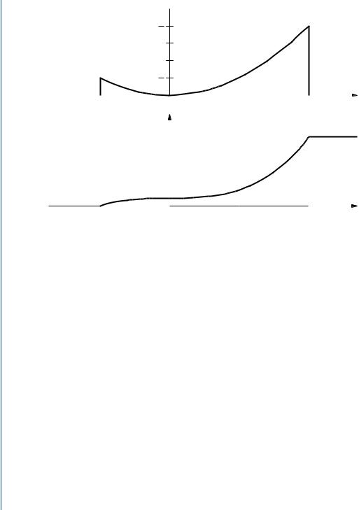
Example 2.3.5. The PDF for the RV x is
βα2, −1 < α < 2 fx (α) = 0, otherwise.
Find β so that fx is a PDF, and find the CDF Fx .
Solution. We require
∞ |
2 |
β |
|
|
|
|
1 = |
fx (α) d α = β α2 d α = |
(8 |
+ 1) |
= 3β |
||
|
||||||
3 |
||||||
−∞ |
−1 |
|
|
|
|
so that β = 1/3. We note that fx (α) ≥ 0, as required. We obtain the CDF using
α
Fx (α) = fx (α ) d α .
−∞
Since fx (α ) = 0 for α < −1 we obtain Fx (α) = 0 for α < −1. For −1 ≤ α < 2 we obtain
|
α |
1 |
|
|||
Fx (α) = |
|
1 |
α 2 d α = |
(α3 + 1). |
||
|
|
|
|
|||
|
3 |
9 |
||||
|
−1 |
|
|
|
||
94 BASIC PROBABILITY THEORY FOR BIOMEDICAL ENGINEERS
 fx (α )
4
3
1
3
|
|
|
|
|
|
|
|
|
|
|
|
|
−1 |
0 |
|
1 |
2 |
α |
|||||
|
|
|
1 |
|
|
Fx (α ) |
|
|
|
|
|
|
|
|
|
|
|
|
|
|
|
||
|
|
|
|
|
|
|
|
|
|
|
|
|
|
|
|
|
|
|
|
|
|
||
|
|
|
1 |
|
|
|
|
|
|
|
|
|
|
|
|
|
|
|
|
|
|
|
|
|
|
|
2 |
|
|
|
|
|
|
|
|
|
|
|
|
|
|
|
|
|
|
|
|
|
|
|
|
|
|
|
|
|
|
|
|
|
|
|
|
|
|
|
|
|
|
|
|
|
−1 |
0 |
|
1 |
2 |
α |
|||||
FIGURE 2.5: PDF and CDF for Example 2.3.5 |
|
|
|
|
|
||||||
Finally, since fx (α ) = 0 for α > 2 we have Fx (α) = 1 for α ≥ 2. Note that |
fx (−1) and fx (2) |
||||||||||
could be defined to be any real numbers without affecting the result. In fact, the PDF could be redefined at any discrete set of points without affecting the result.
The PDF and CDF for this example are illustrated in Fig. 2.5. It is extremely important
to be able to visualize the relationship between the PDF and CDF. |
|
||
Example 2.3.6. The RV x has PDF fx (α) = 5e −5α u(α). Find P (−1 < x < 2). |
|||
Solution. We have |
|
|
|
2 |
2 |
2 |
|
P (−1 < x < 2) = fx (α) d α = 5e −5α d α = −e −5α |
|||
0 = 1 − e −10. |
|||
−1 |
0 |
|
|
2.3.3Mixed Random Variables
Mixed random variables are neither discrete nor continuous. The resulting CDF is piecewise continuous. Probabilities for mixed random variables can be found in several ways. Splitting the CDF into the sum of a jump CDF and a continuous CDF and using the corresponding PMF and PDF is one approach, and is treated in this section.

RANDOM VARIABLES 95
Definition 2.3.6. A RV x defined on (S, F, P ) is a mixed RV if it is neither discrete nor continuous.
Theorem 2.3.4 (Lebesgue Decomposition Theorem). A CDF Fmay be expressed as
F(α) = γ FC (α) + (1 − γ )FD(α), |
(2.38) |
where 0 ≤ γ ≤ 1, FC is a continuous CDF, and FD is a discrete CDF.
Proof. Note that if F is continuous then γ = 1 and FC = F. Similarly, if F is discrete then γ = 0 and FD = F.
Assume F is neither continuous nor discrete. Define
q (α) = F(α) − F(α−).
Then q (α) ≥ 0, and q (α) = 0 only at isolated points, say α D. Let
(1 − γ )FD(α) = q (α )
α ≤α
and
1 − γ = q (α ).
α D
Then FD is a monotone nondecreasing, right-continuous jump function, with FD(−∞) = 0 and FD(+∞) = 1; i.e., FD is a discrete CDF. Now, let
FC (α) = F(α) − (1 − γ )FD(α) .
γ
Then FC (−∞) = 0, FC (+∞) = 1, and FC is right-continuous since both F and FD are right-continuous. Also,
FC ( |
α |
) − FC |
( |
α− |
) = |
|
q (α) − q (α) |
= 0 |
. |
|
γ |
||||||||||
|
|
|
|
|||||||
Consequently, FC is a continuous CDF. |
|
|
|
|
|
|
|
|||
Although the above decomposition theorem is useful, there is no guarantee that FC is absolutely continuous and hence that FC is the CDF of a continuous RV. It can be shown that FC can always be further decomposed into the sum of an absolutely continuous part and a singular part [4]. We will assume throughout that the singular part is zero, and hence that FC is the CDF for a continuous RV. All CDFs arising in practical applications satisfy this assumption. For our purposes then, if γ = 1 the CDF describes a continuous RV and if γ = 0 the CDF describes a discrete RV.
96 BASIC PROBABILITY THEORY FOR BIOMEDICAL ENGINEERS
 Fx (α )
1
|
0.5 |
|
|
|
|
q(α ) |
|
|
|
|
|
0.25 |
|
−1 |
0 |
1 |
α |
−1 |
0 |
α |
 γ FC ( α )
1
(1 − γ )FD (α )
0.5 |
|
0.5 |
|
|
|
|
|
|
|
|
|
|
|
|
|
|
|
|
α |
|
|
|
|
|
|
|
|||
|
−1 |
0 |
|
|
|
1 |
|
|
|
|
|
|
−1 0 α |
||||||||||||
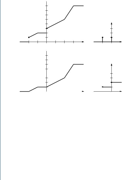
FIGURE 2.6: Plots for Example 2.3.7 |
|
|
|
|
|
|
|
|
|
|
|
|
|
|
|
|
|
|
|
||||||
Example 2.3.7. The RV x has CDF |
|
|
|
|
|
|
|
|
|
|
|
|
|
|
|
|
|
|
|
||||||
|
|
|
0, |
|
1 |
|
|
α < −1 |
1 |
|
|
||||||||||||||
|
|
|
|
1 |
|
+ |
(α + 1), |
−1 ≤ α < − |
|
|
|||||||||||||||
|
|
|
|
|
|
|
|
|
|
|
|
||||||||||||||
|
|
|
|
8 |
|
4 |
2 |
|
|
||||||||||||||||
|
|
|
1 |
|
|
|
|
|
|
|
1 |
≤ α < 0 |
|
|
|
|
|||||||||
|
|
|
|
|
, |
|
|
|
|
|
− |
|
|
|
|
|
|||||||||
|
|
|
4 |
|
|
|
|
|
2 |
|
|
|
|
||||||||||||
|
|
|
Fx (α) = 3 |
+ |
1 |
α, |
0 ≤ α < 1 |
|
|
|
|
||||||||||||||
|
|
|
|
|
|
|
|
|
|
|
|
||||||||||||||
|
|
|
|
8 |
|
4 |
|
|
|
|
|||||||||||||||
|
|
|
5 |
|
|
3 |
|
|
3 |
|
|
|
|
|
|||||||||||
|
|
|
|
|
|
+ |
|
|
(α − 1), |
1 ≤ α < |
|
|
|
|
|
|
|||||||||
|
|
|
8 |
|
4 |
2 |
|
|
|
|
|||||||||||||||
|
|
|
1, |
|
|
|
|
|
|
3 |
≤ α. |
|
|
|
|
||||||||||
|
|
|
|
|
|
|
|
|
|
2 |
|
|
|
|
|||||||||||
Express Fx as Fx = γ FC + (1 − γ )FD, where FC is a continuous CDF and FD is a discrete CDF.
Solution. Plots for this example are given in Fig. 2.6. Following the notation in the proof of
RANDOM VARIABLES 97
 Fx (α )
1
0.5
|
|
|
|
|
|
|
|
|
|
|
|
|
|
|
|
|
|
|
|
|
|
|
|
0 |
1 |
|
|
2 |
3 |
|
|
|
4 |
|
|
|
α |
||||||||||
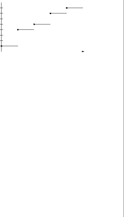
FIGURE 2.7: Cumulative distribution function for Drill Problem 2.3.1 |
|
|
|
||||||||||||||||||||
the Lebesgue Decomposition Theorem, |
|
|
|
|
|
|
|
|
|
|
|
|
|
|
|
|
|
||||||
|
|
|
|
|
|
|
|
|
|
|
1 |
, α = −1, 0 |
|||||||||||
|
q (α) = Fx (α) − Fx (α−) = |
|
|
|
|||||||||||||||||||
|
|
8 |
|||||||||||||||||||||
|
|
|
|
|
|
|
|
|
|
|
0, |
|
|
otherwise. |
|||||||||
Hence, |
|
|
|
|
|
|
|
|
|
|
|
|
|
|
|
|
|
|
|
|
|
||
|
|
|
|
|
|
|
|
|
|
|
0 |
|
|
|
|
α < −1 |
|
|
|
||||
|
(1 − γ )FD(α) = q (α ) |
1 |
, |
|
|
−1 ≤ α < 0 |
|||||||||||||||||
|
8 |
|
|
||||||||||||||||||||
|
|
|
|
|
|
α ≤α |
1 |
, |
|
|
|
0 ≤ α; |
|
|
|
||||||||
|
|
|
|
|
|
|
|
|
|
|
4 |
|
|
|
|
|
|
||||||
so that 1 − γ = 1/4 and γ = 3/4. Finally, γ FC = Fx − (1 − γ )FD, or |
|||||||||||||||||||||||
|
|
|
0, |
|
|
|
|
|
α < −1 |
1 |
|
||||||||||||
|
|
|
|
1 |
(α + 1), |
|
−1 ≤ α < − |
|
|||||||||||||||
|
|
|
|
|
|
|
|
|
|||||||||||||||
|
|
|
|
4 |
|
2 |
|
||||||||||||||||
|
|
|
1 |
, |
|
|
|
|
|
− |
1 |
≤ α < 0 |
|
|
|
||||||||
|
|
|
|
|
|
|
|
|
|
|
|
|
|
||||||||||
|
γ FC (α) = |
8 |
|
|
|
|
|
2 |
|
|
|
||||||||||||
|
|
1 |
+ |
1 |
α, |
|
0 ≤ α < 1 |
|
|
|
|||||||||||||
|
|
|
|
8 |
|
4 |
|
|
|
|
|||||||||||||
|
|
|
3 |
|
3 |
|
|
|
|
|
|
|
3 |
|
|
|
|
||||||
|
|
|
|
|
+ |
|
|
(α − 1), |
|
1 ≤ α < |
|
|
|
|
|
||||||||
|
|
|
8 |
4 |
|
2 |
|
|
|
||||||||||||||
|
|
|
3 |
, |
|
|
|
|
3 |
|
≤ α. |
|
|
|
|||||||||
|
|
|
|
|
|
|
|
|
|
|
|
|
|
||||||||||
|
|
|
4 |
|
|
|
|
2 |
|
|
|
||||||||||||
Drill Problem 2.3.1. The discrete random variable x has cumulative distribution function Fx shown in Fig. 2.7. Find (a) px (−1), (b) px (0), (c )P (0 ≤ x ≤ 3), (d )P (0 < x ≤ 2).
Answers: 7/8, 1/8, 0, 1/2.

98 BASIC PROBABILITY THEORY FOR BIOMEDICAL ENGINEERS
Drill Problem 2.3.2. A committee of three members is to be formed from four engineers and three physicists. Let x be a RV which assigns to every sample point in S a value equal to the number of engineers on the committee. Determine: (a) px (0), (b) px (1), (c ) px (2), and (d) px (3).
Answers: 1/35, 4/35, 12/35, 18/35.
Drill Problem 2.3.3. The waveform w(t) is uniformly sampled every 0.2 s from t = 0 s to t = 4 s, where
( |
) |
= |
2t, |
0 ≤ t |
≤ 2 |
|
w t |
|
4e −2(t−2), 2 < t |
≤ |
4. |
||
|
|
|
|
|
|
|
The sampled values are rounded off to the nearest integer and collected in the set S. The RV x(ζ ) = ζ for all ζ S. Determine: (a) px (0), (b) px (1), (c ) px (2), (d ) px (3), (e ) px (5).
Answers: 1/3, 5/21, 4/21, 1/7, 0.
Drill Problem 2.3.4. Suppose the RV x has the PMF
|
1 |
, |
α = 0, 2 |
|
|
|
8 |
||
px (α) = |
1 |
, |
α = 1, 3, 4 |
|
|
4 |
|||
|
0, |
otherwise. |
||
Find: (a) Fx (−1), (b)Fx (0), (c )Fx (1), (d )Fx (3).
Answers: 3/8, 1/8, 3/4, 0.
Drill Problem 2.3.5. The PDF for the RV x is
fx |
(α) |
= |
β(α + 1), −1 < α < 2 |
|
|
0, |
otherwise, |
||
where β is a constant. Determine: (a) β, (b)P (x ≤ −1), (c )Fx (0), (d )P (0 ≤ x ≤ 2).
Answers: 0, 1/9, 2/9, 8/9.
Drill Problem 2.3.6. The PDF for the RV x is |
|
||
fx (α) = |
β(α1/2 |
+ |
α−1/2), 0 < α < 1 |
0, |
otherwise, |
||
where β is a constant. Determine: (a) β, (b)P (x ≥ 1/2), (c )Fx (1/4), (d )P (x = 1/4).
Answers: 0.406, 3/8, 0, 0.381.
RANDOM VARIABLES 99
|
|
|
Fx (α ) |
|
|
|
|
1 |
|
|
|
−2 |
−1 |
0 |
1 |
2 |
α |
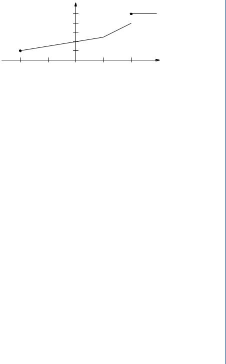
FIGURE 2.8: Cumulative distribution function for Drill Problem 2.3.8
Drill Problem 2.3.7. The CDF for the RV x is
0, α < −1
Fx (α) = 3(α − α3/3 + 2/3)/4, −1 ≤ α < 1 1, 1 ≤ α.
Determine: (a) Fx (0), (b)P (x ≥ 1/2), (c ) fx (0), (d ) fx (4/3).
Answers: 5/32, 1/2, 0, 3/4.
Drill Problem 2.3.8. Random variable x has the mixed CDF Fx shown in Fig. 2.8. Find (a) P (−1 ≤ x < 0.5), (b)P (−2 < x < −1), (c )P (−2 ≤ x < −1), (d )P (x > 1.5).
Answers: 0.1, 0.15, 0.35, 0.3.
2.4RIEMANN-STIELTJES INTEGRATION
We will have a great interest in evaluating integrals of the form
b
d F(α) ,
a
d F(α) ,
B
and
b
g (α) d F(α) ,
a

100 BASIC PROBABILITY THEORY FOR BIOMEDICAL ENGINEERS
where F is a CDF, a and b are real numbers, B is a Borel set, and g : R →R . Such integrals are known as Riemann-Stieltjes integrals. In the following we assume that F is the CDF for the RV x and that a < b. In the special case that B = (a, b] and g (α) = 1 for all α, then all the above integrals are the same. We establish below that
b |
|
P ({ζ : a < x(ζ ) ≤ b}) = F(b) − F(a) = d F(α) . |
(2.39) |
a
The Riemann-Stieltjes integral provides a unified framework for treating continuous, discrete, and mixed RVs—all with one kind of integration. An important alternative is to use a standard Riemann integral for continuous RVs, a summation for discrete RVs, and a Riemann integral with an integrand containing Dirac delta functions for mixed RVs.
We begin with a brief review of the standard Riemann integral. Let
a = α0 < α1 < α2 < · · · < αn = b, |
|
(2.40) |
|||||||||
αi−1 ≤ ξi ≤ αi , |
|
i = 1, 2, . . . , n, |
|
(2.41) |
|||||||
and |
|
|
|
|
|
|
|
|
|
|
|
|
|
n = |
1maxi n{αi − αi−1}. |
|
|
(2.42) |
|||||
|
|
|
|
|
≤ ≤ |
|
|
|
|
|
|
The Riemann integral is defined by |
|
|
|
|
|
|
|
|
|||
b |
|
|
|
|
|
n |
|
|
|
|
|
h( |
|
) d |
|
= n →0 |
|
i i − |
i−1 |
|
(2.43) |
||
|
|
i 1 h |
), |
||||||||
|
α |
|
α |
|
lim |
|
|
(ξ )(α |
α |
|
|
a |
|
|
|
|
|
= |
|
|
|
|
|
provided the limit exists and is independent of the choice of {ξi }. Note that n → ∞ as n → 0. The summation above is called a Riemann sum. We remind the reader that this is the “usual” integral of calculus and has the interpretation as the area under the curve h between a and b.
With the same notation as above, the Riemann-Stieltjes integral is defined by
b |
n |
|
g ( |
|
) d F( |
|
) = |
n →0 |
i |
|
1 |
g ( |
i )(F( |
i ) − F( |
i−1)) |
|
(2.44) |
|
α |
|
α |
|
lim |
|
|
|
ξ |
|
α |
α |
, |
|
a |
|
|
|
|
|
|
= |
|
|
|
|
|
|
|
provided the limit exists and is independent of the choice of {ξi }.