

Lecture Notes: Introduction to Finite Element Method |
Chapter 3. Two-Dimensional Problems |
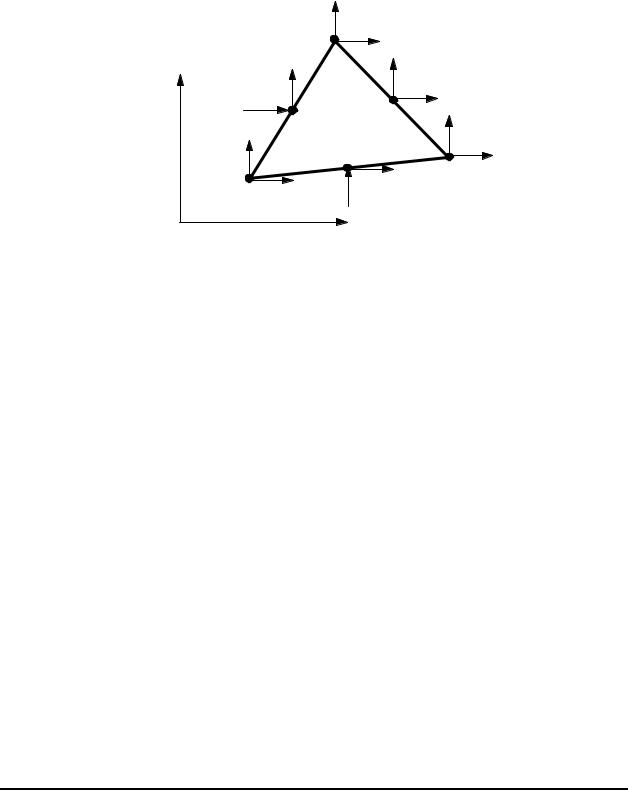
Linear Strain Triangle (LST or T6)
This element is also called quadratic triangular element.
|
|
|
v3 |
u3 |
|
|
|
|
|
3 |
|
|
|
|
|
|
|
|
|
v5 |
|
|
|
y |
v6 |
|
|
|
|
|
|
|
|
|
|
5 |
u5 |
|
|
u6 |
6 |
|
|
|
|
||
|
v1 |
|
|
|
|
v2 |
|
|
|
|
|
|
|
|
|
1 |
u1 |
|
4 |
v4 |
u4 |
2 |
u2 |
|
|
|
|
||||
|
|
|
|
|
|
||
|
|
|
|
x |
|
|
|
Quadratic Triangular Element
There are six nodes on this element: three corner nodes and three midside nodes. Each node has two degrees of freedom (DOF) as before. The displacements (u, v) are assumed to be quadratic functions of (x, y),
u = b + b x + b y + b x2 |
+ b xy + b y2 |
|
|||||
1 |
2 |
3 |
4 |
5 |
6 |
(31) |
|
v = b + b x + b y + b x |
2 + b xy + b y2 |
||||||
|
|||||||
7 |
8 |
9 |
10 |
11 |
12 |
|
|
where bi (i = 1, 2, ..., 12) are constants. From these, the strains are found to be,
εx = b2 + 2b4 x + b5 y |
|
εy = b9 + b11 x + 2b12 y |
(32) |
γ xy = (b3 + b8 ) +(b5 + 2b10 )x +(2b6 + b11 ) y |
|
which are linear functions. Thus, we have the “linear strain triangle” (LST), which provides better results than the CST.
© 1997-2002 Yijun Liu, University of Cincinnati |
91 |
Lecture Notes: Introduction to Finite Element Method |
Chapter 3. Two-Dimensional Problems |
In the natural coordinate system we defined earlier, the six shape functions for the LST element are,
N1 = ξ(2ξ −1) |
|
||
N2 |
= η(2η −1) |
|
|
N3 |
=ζ(2ζ −1) |
(33) |
|
N4 = 4ξη |
|||
|
|||
N5 |
= 4ηζ |
|
|
N6 |
= 4ζ ξ |
|
|
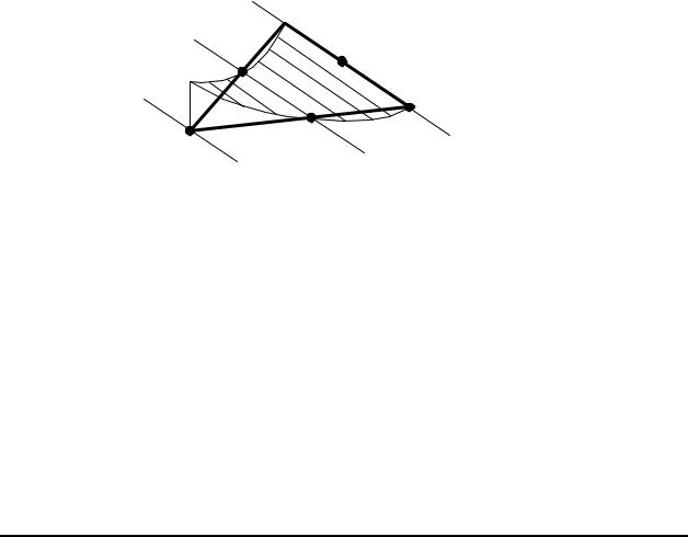
in which ζ =1−ξ −η. Each of these six shape functions
represents a quadratic form on the element as shown in the figure.
ξ=0
3 ξ=1/2 
6 5
ξ=1 |
1 |
N1 |
|
|
1 |
4 |
2 |
Shape Function N1 for LST
Displacements can be written as,
6 |
6 |
|
u = ∑Ni ui , |
v = ∑Ni vi |
(34) |
i=1 |
i=1 |
|
The element stiffness matrix is still given by
k = ∫BT EB dV , but here BTEB is quadratic in x and y. In
V
general, the integral has to be computed numerically.
© 1997-2002 Yijun Liu, University of Cincinnati |
92 |
Lecture Notes: Introduction to Finite Element Method |
Chapter 3. Two-Dimensional Problems |
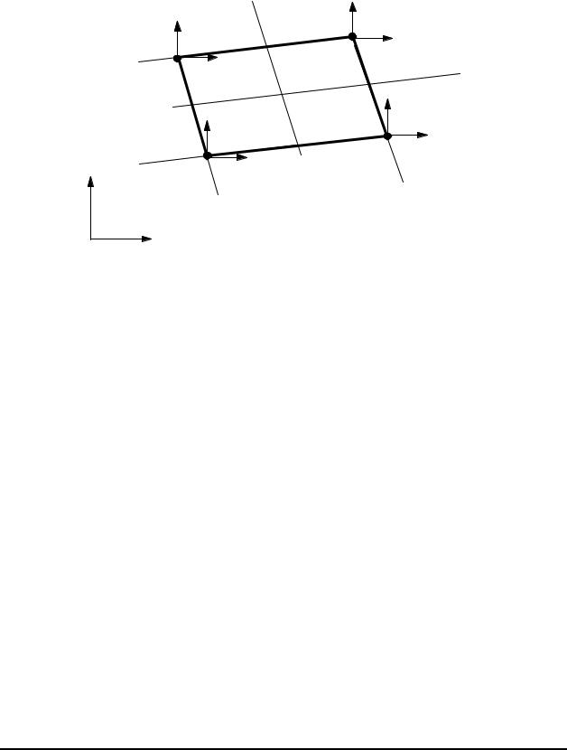
Linear Quadrilateral Element (Q4)
|
|
v4 |
η |
v3 |
u3 |
|
|
|
|
||
η =1 |
4 |
u4 |
3 |
ξ |
|
|
|
||||
|
|
|
v1 |
2 |
v2 |
|
|
|
u2 |
||
|
|
|
1 |
||
y |
η |
= −1 |
u1 |
|
|
|
|
|
|
||
ξ = −1 |
ξ =1 |
x
Linear Quadrilateral Element
There are four nodes at the corners of the quadrilateral shape. In the natural coordinate system (ξ,η), the four shape
functions are,
N1 |
= |
1 |
(1−ξ)(1−η), |
|
N2 |
= |
1 |
(1+ξ)(1−η) |
|
|
4 |
|
|
|
|
4 |
(35) |
|
|
1 |
|
|
|
|
1 |
|
N3 |
= |
(1+ξ)(1+η), |
N4 |
= |
(1−ξ)(1+η) |
|||
|
|
4 |
|
|
|
|
4 |
|
|
|
4 |
|
|
|
|
|
|
Note that ∑Ni =1 at any point inside the element, as expected. |
||||||||
|
|
i=1 |
|
|
|
|
|
|
The displacement field is given by |
||||||||
|
4 |
|
|
4 |
|
|
|
|
u = ∑Ni ui , |
v = ∑Ni vi |
(36) |
||||||
|
i=1 |
|
|
i=1 |
|
|
|
|
which are bilinear functions over the element.
© 1997-2002 Yijun Liu, University of Cincinnati |
93 |
Lecture Notes: Introduction to Finite Element Method |
Chapter 3. Two-Dimensional Problems |
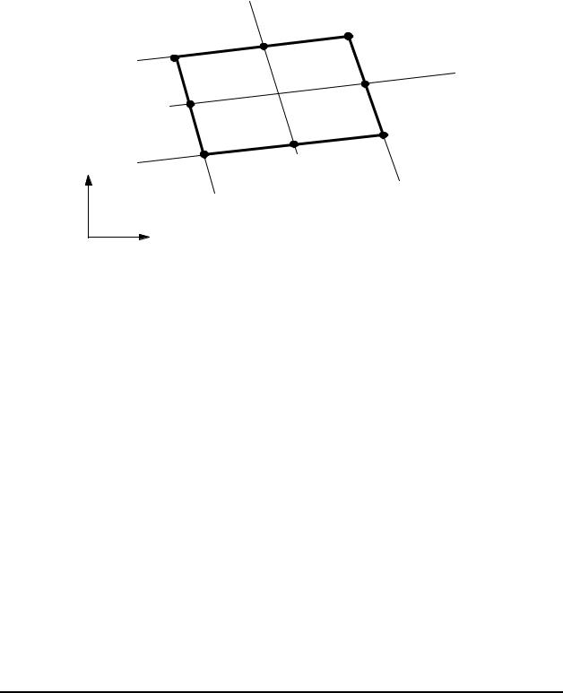
Quadratic Quadrilateral Element (Q8)
This is the most widely used element for 2-D problems due to its high accuracy in analysis and flexibility in modeling.
|
|
η |
|
|
η =1 |
4 |
7 |
3 |
ξ |
|
|
|||
|
|
|
|
8 |
|
6 |
|
5 |
2 |
||
1 |
|||
|
|||
|
|
||
y η = −1 |
|
|
|
ξ = −1 |
|
ξ =1 |
x
Quadratic Quadrilateral Element
There are eight nodes for this element, four corners nodes and four midside nodes. In the natural coordinate system (ξ,η),
the eight shape functions are,
N1 |
= |
1 |
(1−ξ)(η −1)(ξ +η +1) |
|
|
4 |
|
N2 |
= |
1 |
(1+ξ)(η −1)(η −ξ +1) |
|
|
4 |
(37) |
|
|
1 |
|
N3 |
= |
(1+ξ)(1+η)(ξ +η −1) |
|
|
|
4 |
|
N4 |
= |
1 |
(ξ −1)(η +1)(ξ −η +1) |
|
|
4 |
|
© 1997-2002 Yijun Liu, University of Cincinnati |
94 |

Lecture Notes: Introduction to Finite Element Method Chapter 3. Two-Dimensional Problems
N5 |
= |
1 |
(1−η)(1−ξ2 ) |
|
|
2 |
|
N6 |
= |
1 |
(1+ξ)(1−η2 ) |
|
|
2 |
|
N7 |
= |
1 |
(1+η)(1−ξ2 ) |
|
|
2 |
|
N8 |
= |
1 |
(1−ξ)(1−η2 ) |
|
|
2 |
|
8 |
|
Again, we have ∑Ni |
=1 at any point inside the element. |
i=1 |
|
The displacement field is given by
8 |
8 |
|
u = ∑Ni ui , |
v = ∑Ni vi |
(38) |
i=1 |
i=1 |
|
which are quadratic functions over the element. Strains and stresses over a quadratic quadrilateral element are linear functions, which are better representations.
Notes:
•Q4 and T3 are usually used together in a mesh with linear elements.
•Q8 and T6 are usually applied in a mesh composed of quadratic elements.
•Quadratic elements are preferred for stress analysis, because of their high accuracy and the flexibility in modeling complex geometry, such as curved boundaries.
© 1997-2002 Yijun Liu, University of Cincinnati |
95 |