

Lecture Notes: Introduction to Finite Element Method |
Chapter 2. Bar and Beam Elements |
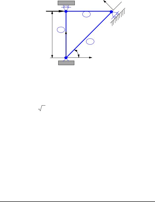
Example 2.4 (Multipoint Constraint)
y’
 x’
x’
P |
|
3 |
|
2 |
2 |
L |
1 |
Y |
|
|
3 |
|
1 |
45o |
|
X |
|
|
|
For the plane truss shown above,
P = 1000 kN, L = 1m, E = 210GPa,
A = 6.0 ×10⁻⁴ m2 |
for elements 1 and 2, |
A = 6 2 ×10⁻⁴ m2 |
for element 3. |
Determine the displacements and reaction forces.
Solution:
We have an inclined roller at node 3, which needs special attention in the FE solution. We first assemble the global FE equation for the truss.
Element 1:
θ = 90o , l = 0, m = 1
© 1997-2002 Yijun Liu, University of Cincinnati |
47 |
Lecture Notes: Introduction to Finite Element Method |
Chapter 2. Bar and Beam Elements |
|
|
|
u1 |
|
|
|
0 |
k1 |
= |
(210 ×109 )(6.0 ×10⁻⁴ ) |
0 |
1 |
|
||
|
|
0 |
|
|
|
|
|
|
|
|
0 |
Element 2:
θ = 0o , l = 1, m = 0
|
|
|
u2 |
|
|
|
|
1 |
|
k2 |
= |
(210 ×109 )(6.0 ×10⁻⁴ ) |
|
0 |
1 |
|
|
||
|
|
−1 |
||
|
|
|
|
0 |
|
|
|
|
|
Element 3:
θ = 45o , l = 12 , m = 12
|
|
|
|
|
u1 |
|
|
|
|
|
0.5 |
k 3 = (210 ×10 |
9 |
|
|
−4 |
|
|
)(6 |
2 ×10 |
|
) 0.5 |
|
|
|
2 |
|
|
− 0.5 |
|
|
|
|
|
|
|
|
|
|
|
− 0.5 |
v1 |
u2 |
v2 |
|
|
0 |
0 |
0 |
|
|
1 |
0 |
−1 |
(N / m) |
|
0 |
0 |
0 |
|
|
|
|
|||
−1 |
0 |
1 |
|
|
|
|
|||
v2 |
u3 |
v3 |
|
0 |
−1 |
0 |
|
0 |
0 |
0 |
(N / m) |
0 |
1 |
|
|
0 |
|
||
0 |
0 |
|
|
0 |
|
v1 |
u3 |
v3 |
|
0.5 |
− 0.5 |
− 0.5 |
|
0.5 |
− 0.5 |
− 0.5 |
|
− 0.5 |
0.5 |
0.5 |
|
|
|||
− 0.5 |
0.5 |
0.5 |
|
|
|||
(N / m)
© 1997-2002 Yijun Liu, University of Cincinnati |
48 |
Lecture Notes: Introduction to Finite Element Method |
Chapter 2. Bar and Beam Elements |
The global FE equation is,
0.5 0.5 |
0 |
0 |
−0.5 |
||
|
15. |
0 |
−1 |
−0.5 |
|
|
|||||
|
1 |
0 |
−1 |
||
1260 ×105 |
|
||||
|
|
|
1 |
0 |
|
|
|
|
15. |
||
|
|
|
|
||
|
|
|
|
|
|
Sym. |
|
|
|
|
|
Load and boundary conditions (BC):
u1 = v1 = v2 = 0, and v3' = 0,
F2 X = P, F3x' = 0.
−0.5 u1 |
|
F1X |
|||
|
|
|
|
|
|
−0.5 v1 |
|
F1Y |
|||
0 |
u2 |
|
F2 X |
||
0 |
v |
2 |
|
= F |
|
|
|
|
2Y |
||
05. |
|
|
|
|
|
u3 |
|
F3 X |
|||
05. |
v3 |
|
F3Y |
||
From the transformation relation and the BC, we have
' |
|
2 |
2 |
u3 |
|
= |
2 |
(−u3 |
+ v3 ) = 0, |
v3 |
= − |
2 |
2 |
|
|
2 |
|||
|
|
v3 |
|
|
|
|
that is,
u3 −v3 = 0
This is a multipoint constraint (MPC).
Similarly, we have a relation for the force at node 3,
|
2 |
2 |
F3 X |
|
2 |
|
F3x' = |
2 |
2 |
F |
= |
2 |
(F3 X + F3Y ) = 0, |
|
|
|
3Y |
|
|
|
that is,
© 1997-2002 Yijun Liu, University of Cincinnati |
49 |

Lecture Notes: Introduction to Finite Element Method |
Chapter 2. Bar and Beam Elements |
F3 X + F3Y = 0
Applying the load and BC’s in the structure FE equation by ‘deleting’ 1st, 2nd and 4th rows and columns, we have
|
1 |
−1 0 u |
2 |
|
P |
|
|
1260 ×105 |
−1 |
15. |
|
|
|
|
|
0.5 u3 |
|
= F3 X |
|||||
|
0 |
0.5 |
0.5 v |
3 |
|
F |
|
|
|
|
|
|
3Y |
||
Further, from the MPC and the force relation at node 3, the equation becomes,
1 1260 ×105 −1
0
which is
1 1260 ×105 −1
0 The 3rd equation yields,
−1 |
0 u2 |
|
|
P |
|
|
15. |
|
|
|
|
F3 X |
|
0.5 u3 |
|
= |
|
|||
0.5 |
0.5 u |
3 |
|
− F |
|
|
|
|
|
|
3 X |
||
−1 |
|
|
|
|
P |
|
|
2 |
u2 |
|
= |
|
F |
|
|
|
|
|
|
|
|
3 X |
|
1 |
|
|
|
− F |
|
||
u3 |
|
||||||
|
|
|
|
|
|
3 X |
|
F3 X = −1260 ×105 u3
Substituting this into the 2nd equation and rearranging, we have
1260 ×105 |
1 |
−1 u |
2 |
|
P |
|||
−1 |
3 |
|
|
= |
0 |
|
||
|
u3 |
|
|
|||||
Solving this, we obtain the displacements,
© 1997-2002 Yijun Liu, University of Cincinnati |
50 |

Lecture Notes: Introduction to Finite Element Method Chapter 2. Bar and Beam Elements
u2 |
|
|
1 |
3P |
|
0.01191 |
|
||||
|
u |
|
|
= |
|
|
P |
|
= |
|
(m) |
|
2520 ×105 |
||||||||||
|
3 |
|
|
|
|
0.003968 |
|
||||
|
|
|
|
|
|
|
|||||
From the global FE equation, we can calculate the reaction forces,
F1XF1Y
F2Y
F3 X
F
3Y
|
0 |
−0.5 |
−0.5 |
|
−500 |
|
||||
|
|
0 |
−0.5 |
|
|
|
|
−500 |
|
|
|
|
−0.5 u2 |
|
|
|
|||||
= 1260 ×105 0 |
0 |
0 |
|
|
0.0 |
(kN) |
||||
|
u3 |
|
= |
|
||||||
|
|
|
15. |
05. |
|
|
|
|
|
|
|
−1 |
v3 |
|
−500 |
|
|||||
|
|
0 |
05. |
05. |
|
|
|
500 |
|
|
|
|
|
|
|
|
|
||||
Check the results!
A general multipoint constraint (MPC) can be described as,
∑Aj uj = 0
j
where Aj’s are constants and uj’s are nodal displacement components. In the FE software, such as MSC/NASTRAN, users only need to specify this relation to the software. The software will take care of the solution.
Penalty Approach for Handling BC’s and MPC’s
© 1997-2002 Yijun Liu, University of Cincinnati |
51 |