Построение периодического тренда

После того, как мы определили длину периода (m=14) можно произвести оценку коэффициентов периодического тренда с помощью МНК, используя следующие формулы:

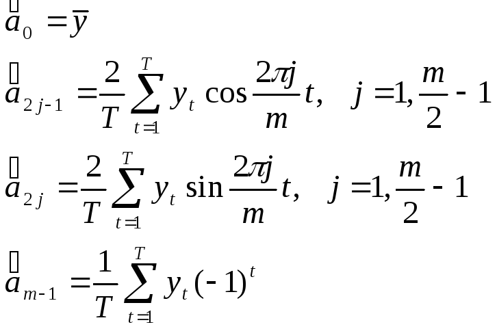
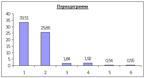
или сделать это, используя статистические пакеты (например ППП «Statgraphics»). Результаты расчетов можно посмотреть в Приложении №7 . В итоге получаем:

j =	1	2	3	4	5	6
A2j-1 =	-5,4915	-3,4956	-0,0397	0,4497	0,0386	0,1922
A2j =	1,8310	3,6666	-1,3575	1,3088	0,7354	0,7131
Rj =	33,5094	25,6631	1,8443	1,9153	0,5422	0,5454
m/j =	14	7	4,6667	3,5	2,8	2,3333

Дисперсионный анализ

Оценим параметры построенного периодического тренда. Следует заметить, что параметры a₀ и a_m-1 проверяются по критерию Стьюдента с (T-m) степенями свободы:

Коэффициенты a_2j-1 и a_2j проверяются на значимость парами (для каждого j) по критерию ²:

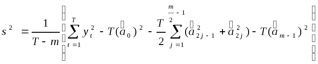
Расчеты приведены в Приложении № 8. В итоге получаем следующий вид периодического тренда:

З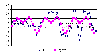 начимыми оказались лишь гармоники 1 и 2

Теперь стоит проверить гипотезу о том, что тренд не содержит периодической составляющей. Для этого определяем расчетное значение F-статистики.

F^P=1,393 F_табл(0,05;13;28)=2,09

Так как F^P < F_табл , то гипотеза об отсутствии в тренде периодической составляющей принимается. Следовательно, при построении прогноза использовать построенную периодическую модель не следует  строить прогноз будем только по трендовой модели.

Построение прогноза

Перестроим лучший тренд по исходным 48-ми данным (см Приложение №9). В результате получим:

Теперь сделаем прогноз по этой модели на следующий 1977 год, т.е. на 12 периодов вперед (в реальности прогноз по трендовой модели на столь длинный период времени делать не следует). Расчет точечных прогнозных значений и доверительных интервалов смотрите в Приложении №9

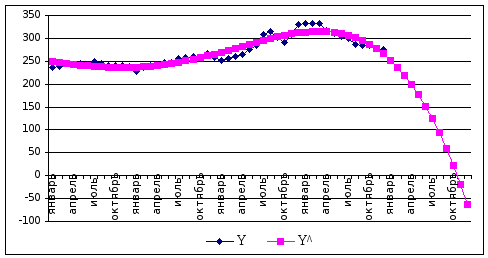
Как видно из графика, построенная модель тренда достаточно хорошо описывает исходную статистику (R² =89,13%). Однако прогноз полученный по этой модели явно искаженный. Это еще раз подтверждает сделанное выше замечание (по поводу величины прогнозного периода). Поэтому прогнозы по трендовой модели стоит строить не более, чем на три периода вперед. Также следует заметить, что в остатках имеется положительная автокорреляция (см. статистику Дарбина-Уотсона в Приложении №9), т.е. есть возможность построения авторегрессионной модели, что поможет более точно построить прогнозные значения.

Приложения

Приложение №1

Вариант №14

Период	Год	Месяц	Y
1	1973	январь	236
2		февраль	238
3		март	245
4		апрель	243
5		май	245
6		июнь	244
7		июль	249
8		август	246
9		сентябрь	241
10		октябрь	240
11		ноябрь	240
12		декабрь	238
13	1974	январь	228
14		февраль	237
15		март	241
16		апрель	244
17		май	247
18		июнь	248
19		июль	256
20		август	259
21		сентябрь	261
22		октябрь	257
23		ноябрь	267
24		декабрь	259
25	1975	январь	251
26		февраль	257
27		март	260
28		апрель	265
29		май	276
30		июнь	285
31		июль	309
32		август	314
33		сентябрь	301
34		октябрь	292
35		ноябрь	309
36		декабрь	331
37	1976	январь	333
38		февраль	332
39		март	333
40		апрель	318
41		май	311
42		июнь	304
43		июль	299
44		август	286
45		сентябрь	285
46		октябрь	284
47		ноябрь	279
48		декабрь	275

Приложение №2

STAT. T-test for Independent Samples (lab_2.sta)

BASIC Note: Variables were treated as independent samples

STATS

Group 1 vs. Group 2	Mean Group 1	Mean Group 2	t-value	df	p
Y1 vs. Y2	252,0000*	305,0588*	-9,98358*	46*	,000000*

Group 1 vs. Group 2	Valid N Group 1	Valid N Group 2	Std.Dev. Group 1	Std.Dev. Group 2	F-ratio variancs	p variancs
Y1 vs. Y2	31*	17*	16,31972*	19,80363*	1,472530*	,350582*

t_табл (0,05;46)=2,013

F_табл(0,05;16;30)=1,99

Приложение №3

Regression Analysis - Linear model: Y = a + b*X

-----------------------------------------------------------------------------

Dependent variable: Y42

Independent variable: t

-----------------------------------------------------------------------------

Standard T

Parameter Estimate Error Statistic P-Value

-----------------------------------------------------------------------------

Intercept 218,35 4,85021 45,0185 0,0000

Slope 2,34697 0,196514 11,9431 0,0000

-----------------------------------------------------------------------------

Analysis of Variance

-----------------------------------------------------------------------------

Source Sum of Squares Df Mean Square F-Ratio P-Value

-----------------------------------------------------------------------------

Model 33988,9 1 33988,9 142,64 0,0000

Residual 9531,61 40 238,29

-----------------------------------------------------------------------------

Total (Corr.) 43520,5 41

Correlation Coefficient = 0,883734

R-squared = 78,0986 percent

Standard Error of Est. = 15,4366

Regression Analysis - Exponential model: Y = exp(a + b*X)

-----------------------------------------------------------------------------

Dependent variable: Y42

Independent variable: t

-----------------------------------------------------------------------------

Standard T

Parameter Estimate Error Statistic P-Value

-----------------------------------------------------------------------------

Intercept 5,40466 0,0167025 323,585 0,0000

Slope 0,00848959 0,000676726 12,5451 0,0000

-----------------------------------------------------------------------------

Analysis of Variance

-----------------------------------------------------------------------------

Source Sum of Squares Df Mean Square F-Ratio P-Value

-----------------------------------------------------------------------------

Model 0,444727 1 0,444727 157,38 0,0000

Residual 0,113033 40 0,00282583

-----------------------------------------------------------------------------

Total (Corr.) 0,55776 41

Correlation Coefficient = 0,892941

R-squared = 79,7344 percent

Standard Error of Est. = 0,0531585

Regression Analysis - Reciprocal-Y model: Y = 1/(a + b*X)

-----------------------------------------------------------------------------

Dependent variable: Y42

Independent variable: t

-----------------------------------------------------------------------------

Standard T

Parameter Estimate Error Statistic P-Value

-----------------------------------------------------------------------------

Intercept 0,00443475 0,0000583415 76,0137 0,0000

Slope -0,0000309286 0,00000236379 -13,0843 0,0000

-----------------------------------------------------------------------------

Analysis of Variance

-----------------------------------------------------------------------------

Source Sum of Squares Df Mean Square F-Ratio P-Value

-----------------------------------------------------------------------------

Model 0,00000590257 10,00000590257 171,20 0,0000

Residual 0,00000137911 40 3,44778E-8

-----------------------------------------------------------------------------

Total (Corr.) 0,00000728169 41

Correlation Coefficient = -0,900336

R-squared = 81,0605 percent

Standard Error of Est. = 0,000185682

Regression Analysis - Square root-X model: Y = a + b*sqrt(X)

-----------------------------------------------------------------------------

Dependent variable: Y42

Independent variable: t

-----------------------------------------------------------------------------

Standard T

Parameter Estimate Error Statistic P-Value

-----------------------------------------------------------------------------

Intercept 191,089 9,19687 20,7776 0,0000

Slope 17,6924 1,98345 8,92005 0,0000

-----------------------------------------------------------------------------

Analysis of Variance

-----------------------------------------------------------------------------

Source Sum of Squares Df Mean Square F-Ratio P-Value

-----------------------------------------------------------------------------

Model 28961,1 1 28961,1 79,57 0,0000

Residual 14559,3 40 363,983

-----------------------------------------------------------------------------

Total (Corr.) 43520,5 41

Correlation Coefficient = 0,815757

R-squared = 66,546 percent

Standard Error of Est. = 19,0783

Regression Analysis - Square root-Y model: Y = (a + b*X)^2

-----------------------------------------------------------------------------

Dependent variable: Y42

Independent variable: t

-----------------------------------------------------------------------------

Standard T

Parameter Estimate Error Statistic P-Value

-----------------------------------------------------------------------------

Intercept 14,8511 0,142078 104,528 0,0000

Slope 0,0705143 0,00575652 12,2495 0,0000

-----------------------------------------------------------------------------

Analysis of Variance

-----------------------------------------------------------------------------

Source Sum of Squares Df Mean Square F-Ratio P-Value

-----------------------------------------------------------------------------

Model 30,6813 1 30,6813 150,05 0,0000

Residual 8,17901 40 0,204475

-----------------------------------------------------------------------------

Total (Corr.) 38,8603 41

Correlation Coefficient = 0,888554

R-squared = 78,9528 percent

Standard Error of Est. = 0,452189

Polynomial Regression Analysis

-----------------------------------------------------------------------------

Dependent variable: Y42

-----------------------------------------------------------------------------

Standard T

Parameter Estimate Error Statistic P-Value

-----------------------------------------------------------------------------

CONSTANT 228,782 8,28757 27,6054 0,0000

t 6,45191 2,60344 2,47823 0,0179

t^2 -0,806261 0,242163 -3,32941 0,0020

t^3 0,0352464 0,00841485 4,18859 0,0002

t^4 -0,000442188 0,0000971212 -4,55295 0,0001

-----------------------------------------------------------------------------

Analysis of Variance

-----------------------------------------------------------------------------

Source Sum of Squares Df Mean Square F-Ratio P-Value

-----------------------------------------------------------------------------

Model 40356,6 4 10089,1 117,99 0,0000

Residual 3163,91 37 85,511

-----------------------------------------------------------------------------

Total (Corr.) 43520,5 41

R-squared = 92,7301 percent

R-squared (adjusted for d.f.) = 91,9441 percent

Standard Error of Est. = 9,24722

Mean absolute error = 7,07397

Durbin-Watson statistic = 0,747583

Приложение №4

t	Y		a+b*t	exp(a+b*t)	1/(a+b*t)	полином 4	a+b*sqrt(t)
1	236		220,70	224,34	227,08	234,46	208,78
2	238		223,04	226,25	228,68	238,74	216,11
3	245		225,39	228,18	230,31	241,80	221,73
4	243		227,74	230,12	231,96	243,83	226,47
5	245		230,08	232,09	233,64	245,01	230,65
6	244		232,43	234,06	235,34	245,51	234,43
7	249		234,78	236,06	237,07	245,47	237,90
8	246		237,13	238,07	238,82	245,03	241,13
9	241		239,47	240,10	240,59	244,34	244,17
10	240		241,82	242,15	242,40	243,50	247,04
11	240		244,17	244,21	244,23	242,63	249,77
12	238		246,51	246,30	246,09	241,84	252,38
13	228		248,86	248,40	247,97	241,21	254,88
14	237		251,21	250,51	249,89	240,81	257,29
15	241		253,55	252,65	251,84	240,72	259,61
16	244		255,90	254,80	253,81	241,00	261,86
17	247		258,25	256,98	255,82	241,69	264,04
18	248		260,60	259,17	257,86	242,83	266,15
19	256		262,94	261,38	259,94	244,44	268,21
20	259		265,29	263,61	262,04	246,54	270,21
21	261		267,64	265,85	264,18	249,13	272,17
22	257		269,98	268,12	266,36	252,21	274,07
23	267		272,33	270,40	268,57	255,76	275,94
24	259		274,68	272,71	270,82	259,76	277,76
25	251		277,02	275,04	273,11	264,16	279,55
26	257		279,37	277,38	275,44	268,92	281,30
27	260		281,72	279,75	277,80	273,98	283,02
28	265		284,07	282,13	280,21	279,26	284,71
29	276		286,41	284,54	282,66	284,70	286,37
30	285		288,76	286,96	285,15	290,18	287,99
31	309		291,11	289,41	287,69	295,63	289,60
32	314		293,45	291,88	290,27	300,92	291,17
33	301		295,80	294,36	292,90	305,93	292,72
34	292		298,15	296,87	295,58	310,52	294,25
35	309		300,49	299,40	298,31	314,56	295,76
36	331		302,84	301,96	301,09	317,89	297,24
37	333		305,19	304,53	303,92	320,34	298,71
38	332		307,53	307,13	306,80	321,73	300,15
39	333		309,88	309,75	309,74	321,89	301,58
40	318		312,23	312,39	312,73	320,61	302,99
41	311		314,58	315,05	315,79	317,69	304,38
42	304		316,92	317,74	318,90	312,90	305,75
43	299		319,27	320,45	322,08	306,02	307,11
44	286		321,62	323,18	325,32	296,81	308,45
45	285		323,96	325,93	328,63	285,02	309,77
46	284		326,31	328,71	332,00	270,39	311,08
47	279		328,66	331,51	335,45	252,64	312,38
48	275		331,00	334,34	338,96	231,50	313,67
		Кт =	0,148	0,156	0,167	0,078	0,096

Приложение №5

Periodogram for RESID

Cumulative Integrated

Frequency Period Ordinate Sum Periodogram

--------------------------------------------------------------------------------

0,0 0,0 0,0 0,0

0,0238095 42,0 4,22049 4,22049 0,00133395

0,047619 21,0 578,705 582,926 0,184243

0,0714286 14,0 703,654 1286,58 0,406643

0,0952381 10,5 140,974 1427,55 0,4512

0,119048 8,4 328,142 1755,7 0,554914

0,142857 7,0 538,896 2294,59 0,72524

0,166667 6,0 204,965 2499,56 0,790023

0,190476 5,25 126,583 2626,14 0,830031

0,214286 4,66667 38,7352 2664,88 0,842274

0,238095 4,2 225,646 2890,52 0,913593

0,261905 3,81818 70,3745 2960,9 0,935836

0,285714 3,5 40,22 3001,12 0,948548

0,309524 3,23077 27,9011 3029,02 0,957366

0,333333 3,0 30,4306 3059,45 0,966984

0,357143 2,8 11,3861 3070,83 0,970583

0,380952 2,625 7,06397 3077,9 0,972816

0,404762 2,47059 22,7291 3100,63 0,98

0,428571 2,33333 11,4533 3112,08 0,98362

0,452381 2,21053 27,059 3139,14 0,992172

0,47619 2,1 7,40308 3146,54 0,994512

0,5 2,0 17,3635 3163,91 1,0

The StatAdvisor

---------------

This table shows the periodogram ordinates for RESID. It is often

used to identify cycles of fixed frequency in the data. The

periodogram is constructed by fitting a series of sine functions at

each of 22 frequencies. The ordinates are equal to the squared

amplitudes of the sine functions. The periodogram can be thought of

as an analysis of variance by frequency, since the sum of the

ordinates equals the total corrected sum of squares in an ANOVA table.

You can plot the periodogram ordinates by selecting Periodogram from

the list of Graphical Options.

Приложение №6

Период			k	Ck		cos	j	Uj
1	1,54		0	87,89	1,000	##	0	45,700
2	-0,74		1	53,90	0,972	##	1	54,131
3	3,20		2	9,62	0,895	##	2	63,822
4	-0,83		3	-13,71	0,784	##	3	62,546
5	-0,01		4	-17,70	0,650	##	4	56,2904
6	-1,51		5	-18,82	0,508	##	5	47,474
7	3,53		6	-18,03	0,370	##	6	40,397
8	0,97		7	-11,37	0,250	##	7	36,935
9	-3,34		8	-11,66	0,157	##	8	33,367
10	-3,50		9	-22,39	0,091	##	9	30,386
11	-2,63		10	-32,40	0,047	##	10	29,229
12	-3,84		11	-24,57	0,020	##	11	28,979
13	-13,21		12	-4,51	0,006	##	12	28,957
14	-3,81		13	4,98	0,001	##	13	28,813
15	0,28		14	10,90	0,000	##	14	28,701
16	3,00
17	5,31
18	5,17
19	11,56
20	12,46
21	11,87
22	4,79
23	11,24
24	-0,76
25	-13,16
26	-11,92
27	-13,98
28	-14,26
29	-8,70
30	-5,18
31	13,37
32	13,08
33	-4,93
34	-18,52
35	-5,56
36	13,11
37	12,66
38	10,27
39	11,11
40	-2,61
41	-6,69
42	-8,90

Приложение №7

Multiple Regression Analysis

-----------------------------------------------------------------------------

Dependent variable: RESID

-----------------------------------------------------------------------------

Standard T

Parameter Estimate Error Statistic P-Value

-----------------------------------------------------------------------------

CONSTANT -0,00081512 1,23793 -0,000658452 0,9995

a1 -5,49196 1,75087 -3,1367 0,0040

a2 1,83036 1,75045 1,04565 0,3047

a3 -3,49596 1,75087 -1,9967 0,0557

a4 3,66606 1,75045 2,09435 0,0454

a5 -0,0392238 1,75087 -0,0224024 0,9823

a6 -1,35751 1,75045 -0,775522 0,4445

a7 0,450862 1,75087 0,257507 0,7987

a8 1,30846 1,75045 0,747498 0,4610

a9 0,0403022 1,75087 0,0230184 0,9818

a10 0,735162 1,75045 0,419984 0,6777

a11 0,192437 1,75087 0,109909 0,9133

a12 0,712703 1,75045 0,407154 0,6870

a13 -0,644543 1,23793 -0,52066 0,6067

-----------------------------------------------------------------------------

Analysis of Variance

-----------------------------------------------------------------------------

Source Sum of Squares Df Mean Square F-Ratio P-Value

-----------------------------------------------------------------------------

Model 1361,71 13 104,747 1,63 0,1363

Residual 1802,2 28 64,3642

-----------------------------------------------------------------------------

Total (Corr.) 3163,91 41

R-squared = 43,0388 percent

R-squared (adjusted for d.f.) = 16,5926 percent

Standard Error of Est. = 8,02273

Mean absolute error = 5,32326

Durbin-Watson statistic = 0,891393

Приложение №8

t						tрасч	tтабл	P-value
1	1,54			a0	-0,001	0,00	2,05	1,00
2	-0,74			a13	-0,64	-0,52	2,05	0,61
3	3,20		j		Rj^2	Хи:2	Хи:2 табл	P-value
4	-0,83		1	a1+a2	33,51	10,93	5,99	0,00
5	-0,01		2	a3+a4	25,66	8,37	5,99	0,02
6	-1,51		3	a5+a6	1,84	0,60	5,99	0,74
7	3,53		4	a7+a8	1,92	0,62	5,99	0,73
8	0,97		5	a9+a10	0,54	0,18	5,99	0,92
9	-3,34		6	a11+a12	0,55	0,18	5,99	0,91
10	-3,50
11	-2,63			s^2 =	64,3617
12	-3,84
13	-13,21
14	-3,81		j		Rj^2	Хи:2	Хи:2 табл	P-value
15	0,28		1	a1+a2	33,51	10,26	5,99	0,01
16	3,00		2	a3+a4	25,66	7,85	5,99	0,02
17	5,31
18	5,17			s^2 =	68,6173
19	11,56
20	12,46
21	11,87				Вывод: гармоники j=1,2 значимы
22	4,79
23	11,24
24	-0,76
25	-13,16		Fр =	1,39303		F(0,05;13;28) =	2,08893
26	-11,92
27	-13,98
28	-14,26
29	-8,70
30	-5,18
31	13,37
32	13,08
33	-4,93
34	-18,52
35	-5,56
36	13,11
37	12,66
38	10,27
39	11,11
40	-2,61
41	-6,69
42	-8,90

Приложение №9

Multiple Regression Analysis

-----------------------------------------------------------------------------

Dependent variable: Y48

-----------------------------------------------------------------------------

Standard T

Parameter Estimate Error Statistic P-Value

-----------------------------------------------------------------------------

CONSTANT 235,622 8,15259 28,9015 0,0000

t 3,41011 2,25467 1,51247 0,1377

t2 -0,48587 0,184415 -2,63465 0,0117

t3 0,023581 0,00562733 4,19044 0,0001

t4 -0,000306782 0,0000569923 -5,38286 0,0000

-----------------------------------------------------------------------------

Analysis of Variance

-----------------------------------------------------------------------------

Source Sum of Squares Df Mean Square F-Ratio P-Value

-----------------------------------------------------------------------------

Model 40945,6 4 10236,4 104,10 0,0000

Residual 4228,29 43 98,3323

-----------------------------------------------------------------------------

Total (Corr.) 45173,9 47

R-squared = 90,64 percent

R-squared (adjusted for d.f.) = 89,7693 percent

Standard Error of Est. = 9,91627

Mean absolute error = 7,4022

Durbin-Watson statistic = 0,65469

Multiple Regression Analysis

-----------------------------------------------------------------------------

Dependent variable: Y48

-----------------------------------------------------------------------------

Standard T

Parameter Estimate Error Statistic P-Value

-----------------------------------------------------------------------------

CONSTANT 252,514 5,36506 47,0663 0,0000

t -2,36238 0,566854 -4,16752 0,0001

t3 0,00894824 0,0009649 9,27375 0,0000

t4 -0,000162524 0,0000168487 -9,64607 0,0000

-----------------------------------------------------------------------------

Analysis of Variance

-----------------------------------------------------------------------------

Source Sum of Squares Df Mean Square F-Ratio P-Value

-----------------------------------------------------------------------------

Model 40263,1 3 13421,0 120,25 0,0000

Residual 4910,85 44 111,61

-----------------------------------------------------------------------------

Total (Corr.) 45173,9 47

R-squared = 89,129 percent

R-squared (adjusted for d.f.) = 88,3878 percent

Standard Error of Est. = 10,5646

Mean absolute error = 8,14179

Durbin-Watson statistic = 0,5614

Regression Results for Y48

------------------------------------------------------------------------------------------------------

Fitted Stnd. Error Lower 95,0% CL Upper 95,0% CL Lower 95,0% CL Upper 95,0% CL

Row Value for Forecast for Forecast for Forecast for Mean for Mean

------------------------------------------------------------------------------------------------------

49 252,592 12,9741 226,444 278,739 237,414 267,77

50 237,152 13,9543 209,029 265,275 218,778 255,525

51 219,52 15,2127 188,861 250,179 197,46 241,58

52 199,553 16,7727 165,75 233,357 173,298 225,808

53 177,105 18,6517 139,515 214,695 146,126 208,084

54 152,023 20,8625 109,977 194,069 115,767 188,279

55 124,153 23,4153 76,9624 171,344 82,0386 166,267

56 93,336 26,3194 40,2927 146,379 44,7534 141,919

57 59,4093 29,5842 -0,213884 119,033 3,71734 115,101

58 22,2061 33,22 -44,7446 89,1568 -41,2688 85,681

59 -18,4442 37,2382 -93,4931 56,6046 -90,4095 53,521

60 -62,7162 41,6514 -146,659 21,2268 -143,914 18,4817

------------------------------------------------------------------------------------------------------