

Chapter 28Digital Signal Processors |
513 |
|||||||
|
|
|
|
|
|
|
|
|
|
|
PM Data |
|
|
DM Data |
|
|
|
PM address bus |
|
Address |
|
|
Address |
DM address bus |
|
|
|
Generator |
|
|
Generator |
|
|
||
Program |
|
|
|
|
|
|
|
Data |
|
|
|
|
|
|
|
||
Memory |
|
|
|
|
|
|
|
Memory |
|
Program Sequencer |
|
|
|||||
instructions and |
|
|
|
|||||
|
|
|
|
|
|
|
data only |
|
secondary data |
|
Instruction |
|
|
|
|||
|
|
|
|
|
||||
|
|
Cache |
|
|
|
|
||
PM data bus |
|
|
|
|
|
|
DM data bus |
|
|
|
|
|
|
|
|
||
Data
Registers
|
I/O Controller |
|
(DMA) |
Muliplier |
|
|
|
|
|
ALU |
High speed I/O |
|
|
|
|
|
(serial, parallel, |
Shifter |
ADC, DAC, etc.) |
|
|
|
|
FIGURE 28-5
Typical DSP architecture. Digital Signal Processors are designed to implement tasks in parallel. This simplified diagram is of the Analog Devices SHARC DSP. Compare this architecture with the tasks needed to implement an FIR filter, as listed in Table 28-1. All of the steps within the loop can be executed in a single clock cycle.
feature is the use of shadow registers for all the CPU's key registers. These are duplicate registers that can be switched with their counterparts in a single clock cycle. They are used for fast context switching, the ability to handle interrupts quickly. When an interrupt occurs in traditional microprocessors, all the internal data must be saved before the interrupt can be handled. This usually involves pushing all of the occupied registers onto the stack, one at a time. In comparison, an interrupt in the SHARC family is handled by moving the internal data into the shadow registers in a single clock cycle. When the interrupt routine is completed, the registers are just as quickly restored. This feature allows step 4 on our list (managing the sample-ready interrupt) to be handled very quickly and efficiently.
Now we come to the critical performance of the architecture, how many of the operations within the loop (steps 6-12 of Table 28-1) can be carried out at the same time. Because of its highly parallel nature, the SHARC DSP can simultaneously carry out all of these tasks. Specifically, within a single clock cycle, it can perform a multiply (step 11), an addition (step 12), two data moves (steps 7 and 9), update two circular buffer pointers (steps 8 and 10), and
514 |
The Scientist and Engineer's Guide to Digital Signal Processing |
control the loop (step 6). There will be extra clock cycles associated with beginning and ending the loop (steps 3, 4, 5 and 13, plus moving initial values into place); however, these tasks are also handled very efficiently. If the loop is executed more than a few times, this overhead will be negligible. As an example, suppose you write an efficient FIR filter program using 100 coefficients. You can expect it to require about 105 to 110 clock cycles per sample to execute (i.e., 100 coefficient loops plus overhead). This is very impressive; a traditional microprocessor requires many thousands of clock cycles for this algorithm.
Fixed versus Floating Point
Digital Signal Processing can be divided into two categories, fixed point and floating point. These refer to the format used to store and manipulate numbers within the devices. Fixed point DSPs usually represent each number with a minimum of 16 bits, although a different length can be used. For instance, Motorola manufactures a family of fixed point DSPs that use 24 bits. There are four common ways that these 216 ' 65,536 possible bit patterns can represent a number. In unsigned integer, the stored number can take on any integer value from 0 to 65,535. Similarly, signed integer uses two's complement to make the range include negative numbers, from -32,768 to 32,767. With unsigned fraction notation, the 65,536 levels are spread uniformly between 0 and 1. Lastly, the signed fraction format allows negative numbers, equally spaced between -1 and 1.
In comparison, floating point DSPs typically use a minimum of 32 bits to store each value. This results in many more bit patterns than for fixed point, 232 ' 4,294,967,296 to be exact. A key feature of floating point notation is that the represented numbers are not uniformly spaced. In the most common format (ANSI/IEEE Std. 754-1985), the largest and smallest numbers are
± 3.4 × 1038 and ± 1.2 × 10& 38 , respectively. The represented values are unequally spaced between these two extremes, such that the gap between any two numbers is about ten-million times smaller than the value of the numbers.
This is important because it places large gaps between large numbers, but small gaps between small numbers. Floating point notation is discussed in more detail in Chapter 4.
All floating point DSPs can also handle fixed point numbers, a necessity to implement counters, loops, and signals coming from the ADC and going to the DAC. However, this doesn't mean that fixed point math will be carried out as quickly as the floating point operations; it depends on the internal architecture. For instance, the SHARC DSPs are optimized for both floating point and fixed point operations, and executes them with equal efficiency. For this reason, the SHARC devices are often referred to as "32-bit DSPs," rather than just "Floating Point."
Figure 28-6 illustrates the primary trade-offs between fixed and floating point DSPs. In Chapter 3 we stressed that fixed point arithmetic is much
Chapter 28Digital Signal Processors
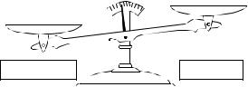
FIGURE 28-6
Fixed versus floating point. Fixed point DSPs are generally cheaper, while floating point devices have better precision, higher dynamic range, and a shorter development cycle.
Precision
Dynamic Range
Development Time
Floating Point
515
Product Cost
Fixed Point
faster than floating point in general purpose computers. However, with DSPs the speed is about the same, a result of the hardware being highly optimized for math operations. The internal architecture of a floating point DSP is more complicated than for a fixed point device. All the registers and data buses must be 32 bits wide instead of only 16; the multiplier and ALU must be able to quickly perform floating point arithmetic, the instruction set must be larger (so that they can handle both floating and fixed point numbers), and so on. Floating point (32 bit) has better precision and a higher dynamic range than fixed point (16 bit) . In addition, floating point programs often have a shorter development cycle, since the programmer doesn't generally need to worry about issues such as overflow, underflow, and round-off error.
On the other hand, fixed point DSPs have traditionally been cheaper than floating point devices. Nothing changes more rapidly than the price of electronics; anything you find in a book will be out-of-date before it is printed. Nevertheless, cost is a key factor in understanding how DSPs are evolving, and we need to give you a general idea. When this book was completed in 1999, fixed point DSPs sold for between $5 and $100, while floating point devices were in the range of $10 to $300. This difference in cost can be viewed as a measure of the relative complexity between the devices. If you want to find out what the prices are today, you need to look today.
Now let's turn our attention to performance; what can a 32-bit floating point system do that a 16-bit fixed point can't? The answer to this question is signal-to-noise ratio. Suppose we store a number in a 32 bit floating point format. As previously mentioned, the gap between this number and its adjacent neighbor is about one ten-millionth of the value of the number. To store the number, it must be round up or down by a maximum of one-half the gap size. In other words, each time we store a number in floating point notation, we add noise to the signal.
The same thing happens when a number is stored as a 16-bit fixed point value, except that the added noise is much worse. This is because the gaps between adjacent numbers are much larger. For instance, suppose we store the number 10,000 as a signed integer (running from -32,768 to 32,767). The gap between numbers is one ten-thousandth of the value of the number we are storing. If we
516 |
The Scientist and Engineer's Guide to Digital Signal Processing |
want to store the number 1000, the gap between numbers is only one onethousandth of the value.
Noise in signals is usually represented by its standard deviation. This was discussed in detail in Chapter 2. For here, the important fact is that the standard deviation of this quantization noise is about one-third of the gap size. This means that the signal-to-noise ratio for storing a floating point number is about 30 million to one, while for a fixed point number it is only about ten-thousand to one. In other words, floating point has roughly 3,000 times less quantization noise than fixed point.
This brings up an important way that DSPs are different from traditional microprocessors. Suppose we implement an FIR filter in fixed point. To do this, we loop through each coefficient, multiply it by the appropriate sample from the input signal, and add the product to an accumulator. Here's the problem. In traditional microprocessors, this accumulator is just another 16 bit fixed point variable. To avoid overflow, we need to scale the values being added, and will correspondingly add quantization noise on each step. In the worst case, this quantization noise will simply add, greatly lowering the signal- to-noise ratio of the system. For instance, in a 500 coefficient FIR filter, the noise on each output sample may be 500 times the noise on each input sample. The signal-to-noise ratio of ten-thousand to one has dropped to a ghastly twenty to one. Although this is an extreme case, it illustrates the main point: when many operations are carried out on each sample, it's bad, really bad. See Chapter 3 for more details.
DSPs handle this problem by using an extended precision accumulator. This is a special register that has 2-3 times as many bits as the other memory locations. For example, in a 16 bit DSP it may have 32 to 40 bits, while in the SHARC DSPs it contains 80 bits for fixed point use. This extended range virtually eliminates round-off noise while the accumulation is in progress. The only round-off error suffered is when the accumulator is scaled and stored in the 16 bit memory. This strategy works very well, although it does limit how some algorithms must be carried out. In comparison, floating point has such low quantization noise that these techniques are usually not necessary.
In addition to having lower quantization noise, floating point systems are also easier to develop algorithms for. Most DSP techniques are based on repeated multiplications and additions. In fixed point, the possibility of an overflow or underflow needs to be considered after each operation. The programmer needs to continually understand the amplitude of the numbers, how the quantization errors are accumulating, and what scaling needs to take place. In comparison, these issues do not arise in floating point; the numbers take care of themselves (except in rare cases).
To give you a better understanding of this issue, Fig. 28-7 shows a table from the SHARC user manual. This describes the ways that multiplication can be carried out for both fixed and floating point formats. First, look at how floating point numbers can be multiplied; there is only one way! That

|
|
|
|
|
|
|
|
|
Chapter 28Digital Signal Processors |
517 |
||||||||||||||||||||||||||||||||||||
|
|
|
Fixed Point |
|
|
|
|
|
|
|
|
|
|
|
|
|
|
|
|
|
|
|
|
|
Floating Point |
|
||||||||||||||||||||
|
|
|
|
|
|
|
|
|
|
|
|
|
|
|
|
|
|
|
|
|
|
|
|
|
|
|
|
|
|
|
|
|
|
|||||||||||||
|
Rn |
|
= Rx * Ry |
|
|
( |
|
S |
|
|
|
|
|
S |
|
|
|
|
|
F |
|
) |
|
|
|
|
|
|
|
|
|
Fn = Fx * Fy |
|
|||||||||||||
|
|
|
|
|
|
|
|
|
|
|
|
|
|
|
|
|||||||||||||||||||||||||||||||
|
MRF |
|
|
|
|
|
|
|
|
|
|
U |
|
|
|
|
|
U |
|
|
|
|
|
I |
|
|
|
|
|
|
|
|
|
|
|
|
|
|
|
|
||||||
|
|
|
|
|
|
|
|
|
|
|
|
|
|
|
|
|
|
|
|
|
|
|
|
|
|
|
|
|
|
|||||||||||||||||
|
MRB |
|
|
|
|
|
|
|
|
|
|
|
|
|
|
|
|
|
|
|
|
FR |
|
|
|
|
|
|
|
|
|
|
F |
|
|
|
|
|
||||||||
|
|
|
|
|
|
|
|
|
|
|
|
|
|
|
|
|
|
|
|
|
|
|
|
|
|
|
|
|
|
|
||||||||||||||||
|
Rn |
|
= MRF |
|
|
+ Rx * Ry |
( |
|
|
|
S |
|
|
|
|
|
|
|
|
S |
|
|
|
|
|
|
|
) |
|
|||||||||||||||||
|
|
|
|
|
|
|
|
|
|
|||||||||||||||||||||||||||||||||||||
|
|
|
|
|
|
|
|
|
||||||||||||||||||||||||||||||||||||||
|
Rn |
|
= MRB |
|
|
|
|
|
|
|
|
|
|
|
|
|
|
|
|
|
|
|
|
U |
|
|
|
|
|
|
|
|
U |
|
|
|
|
|
I |
|
|
|
|
|
||
|
|
|
|
|
|
|
|
|
|
|
|
|
|
|
|
|
|
|
|
|
|
|
|
|
|
|
|
|
|
|
||||||||||||||||
|
MRF |
|
= MRF |
|
|
|
|
|
|
|
|
|
|
|
|
|
|
|
|
|
|
|
|
|
|
|
|
|
|
|
|
|
|
|
|
|
|
|
|
|
FR |
|
|
|
|
|
|
|
|
|
|
|
|
|
|
|
|
|
|
|
|
|
|
|
|
|
|
|
|
|
|
|
|
|
|
|
|
|
|
|
|
|
|
|
|
|
|
|
|||||
|
MRB |
|
= MRB |
|
|
|
|
|
|
|
|
|
|
|
|
|
|
|
|
|
|
|
|
|
|
|
|
|
|
|
|
|
|
|
|
|
|
|
|
|
|
|
|
|
|
|
|
|
|
|
|
|
|
|
|
|
|
|
|
|
|
|
|
|
|
|
|
|
|
|
|
|
|
|
|
|
|
|
|
|
|
|
|
|
|
|
|
|
|
|
|||
|
Rn |
|
= MRF |
|
|
- Rx * Ry ( |
|
S |
|
|
|
|
|
|
S |
|
|
|
|
|
F |
|
|
) |
|
|||||||||||||||||||||
|
|
|
|
|
|
|
|
|
|
|
|
|
||||||||||||||||||||||||||||||||||
|
|
|
|
|
|
|
|
|
|
|
||||||||||||||||||||||||||||||||||||
|
Rn |
|
= MRB |
|
|
|
|
|
|
|
|
|
|
|
|
|
|
|
|
|
|
|
|
U |
|
|
|
|
|
|
U |
|
|
|
|
|
I |
|
|
|
|
|
||||
|
|
|
|
|
|
|
|
|
|
|
|
|
|
|
|
|
|
|
|
|
|
|
|
|
|
|
|
|
|
|
|
|
|
|
||||||||||||
|
MRF |
|
= MRF |
|
|
|
|
|
|
|
|
|
|
|
|
|
|
|
|
|
|
|
|
|
|
|
|
|
|
|
|
|
|
|
|
|
|
|
|
|
FR |
|
|
|
|
|
|
|
|
|
|
|
|
|
|
|
|
|
|
|
|
|
|
|
|
|
|
|
|
|
|
|
|
|
|
|
|
|
|
|
|
|
|
|
|
|
|
|
|
||||
|
MRB |
|
= MRB |
|
|
|
|
|
|
|
|
|
|
|
|
|
|
|
|
|
|
|
|
|
|
|
|
|
|
|
|
|
|
|
|
|
|
|
|
|
|
|
|
|
|
|
|
|
|
|
|
|
|
|
|
|
|
|
|
|
|
|
|
|
|
|
|
|
|
|
|
|
|
|
|
|
|
|
|
|
|
|
|
|
|
|
|
|
|
|
|||
|
Rn |
|
= SAT MRF |
|
|
|
|
|
|
|
|
|
|
|
(SI) |
|
|
|
|
|
|
|
|
|
|
|
|
|
|
|
|
|
|
|
|
|
|
|
||||||||
|
|
|
|
|
|
|
|
|
|
|
|
|
|
|
|
|
|
|
|
|
|
|
|
|
|
|
|
|||||||||||||||||||
|
Rn |
|
= SAT MRB |
|
|
|
|
|
|
|
|
|
|
|
(UI) |
|
|
|
|
|
|
|
|
|
|
|
|
|
|
|
|
|
|
|
|
|
|
|
||||||||
|
MRF |
|
= SAT MRF |
|
|
|
|
|
|
|
|
|
|
|
(SF) |
|
|
|
|
|
|
|
|
|
|
|
|
|
|
|
|
|
|
|
|
|
|
|
||||||||
|
MRB |
|
= SAT MRB |
|
|
|
|
|
|
|
|
|
|
|
(UF) |
|
|
|
|
|
|
|
|
|
|
|
|
|
|
|
|
|
|
|||||||||||||
|
|
|
|
|
|
|
|
|
|
|
|
|
|
|
|
|
|
|
|
|
|
|||||||||||||||||||||||||
|
Rn |
|
= RND MRF |
|
|
|
|
|
|
|
|
|
(SF) |
|
|
|
|
|
|
|
|
|
|
|
|
|
|
|
|
|
|
|
|
|
|
|
||||||||||
|
|
|
|
|
|
|
|
|
|
|
|
|
|
|
|
|
|
|
|
|
|
|
|
|
|
|
|
|||||||||||||||||||
|
Rn |
|
= RND MRB |
|
|
|
|
|
|
|
|
|
(UF) |
|
|
|
|
|
|
|
|
|
|
|
|
|
|
|
|
|
|
|||||||||||||||
|
|
|
|
|
|
|
|
|
|
|
|
|
|
|
|
|
|
|
|
|
|
|
|
|
|
|
||||||||||||||||||||
|
MRF |
|
= RND MRF |
|
|
|
|
|
|
|
|
|
|
|
|
|
|
|
|
|
|
|
|
|
|
|
|
|
|
|
|
|
|
|
|
|
|
|
|
|
|
|||||
|
MRB |
|
= RND MRB |
|
|
|
|
|
|
|
|
|
|
|
|
|
|
|
|
|
|
|
|
|
|
|
|
|
|
|
|
|
|
|
|
|
|
|
|
|
|
|||||
|
|
|
|
|
|
|
|
|
|
|
|
|
|
|
|
|
|
|
|
|
|
|
|
|
|
|
|
|
|
|
|
|
|
|||||||||||||
|
MRF |
|
= 0 |
|
|
|
|
|
|
|
|
|
|
|
|
|
|
|
|
|
|
|
|
|
|
|
|
|
|
|
|
|
|
|
|
|
|
|
|
|
|
|
|
|
|
|
|
|
|
|
|
|
|
|
|
|
|
|
|
|
|
|
|
|
|
|
|
|
|
|
|
|
|
|
|
|
|
|
|
|
|
|
|
|
|
|
|
|
|
|
|
||
|
MRB |
|
|
|
|
|
|
|
|
|
|
|
|
|
|
|
|
|
|
|
|
|
|
|
|
|
|
|
|
|
|
|
|
|
|
|
|
|
|
|
|
|
|
|
|
|
|
|
|
|
|
|
|
|
|
|
|
|
|
|
|
|
|
|
|
|
|
|
|
|
|
|
|
|
|
|
|
|
|
|
|
|
|
|
|
|
|
|
|
|
|
|
|
MRxF = Rn
MRxB
Rn = MRxF
MRxB
FIGURE 28-7
Fixed versus floating point instructions. These are the multiplication instructions used in the SHARC DSPs. While only a single command is needed for floating point, many options are needed for fixed point. See the text for an explanation of these options.
is, Fn = Fx * Fy, where Fn, Fx, and Fy are any of the 16 data registers. It could not be any simpler. In comparison, look at all the possible commands for fixed point multiplication. These are the many options needed to efficiently handle the problems of round-off, scaling, and format.
In Fig. 28-7, Rn, Rx, and Ry refer to any of the 16 data registers, and MRF and MRB are 80 bit accumulators. The vertical lines indicate options. For instance, the top-left entry in this table means that all the following are valid commands: Rn = Rx * Ry, MRF = Rx * Ry, and MRB = Rx * Ry. In other words, the value of any two registers can be multiplied and placed into another register, or into one of the extended precision accumulators. This table also shows that the numbers may be either signed or unsigned (S or U), and may be fractional or integer (F or I). The RND and SAT options are ways of controlling rounding and register overflow.
518 |
The Scientist and Engineer's Guide to Digital Signal Processing |
There are other details and options in the table, but they are not important for our present discussion. The important idea is that the fixed point programmer must understand dozens of ways to carry out the very basic task of multiplication. In contrast, the floating point programmer can spend his time concentrating on the algorithm.
Given these tradeoffs between fixed and floating point, how do you choose which to use? Here are some things to consider. First, look at how many bits are used in the ADC and DAC. In many applications, 12-14 bits per sample is the crossover for using fixed versus floating point. For instance, television and other video signals typically use 8 bit ADC and DAC, and the precision of fixed point is acceptable. In comparison, professional audio applications can sample with as high as 20 or 24 bits, and almost certainly need floating point to capture the large dynamic range.
The next thing to look at is the complexity of the algorithm that will be run. If it is relatively simple, think fixed point; if it is more complicated, think floating point. For example, FIR filtering and other operations in the time domain only require a few dozen lines of code, making them suitable for fixed point. In contrast, frequency domain algorithms, such as spectral analysis and FFT convolution, are very detailed and can be much more difficult to program. While they can be written in fixed point, the development time will be greatly reduced if floating point is used.
Lastly, think about the money: how important is the cost of the product, and how important is the cost of the development? When fixed point is chosen, the cost of the product will be reduced, but the development cost will probably be higher due to the more difficult algorithms. In the reverse manner, floating point will generally result in a quicker and cheaper development cycle, but a more expensive final product.
Figure 28-8 shows some of the major trends in DSPs. Figure (a) illustrates the impact that Digital Signal Processors have had on the embedded market. These are applications that use a microprocessor to directly operate and control some larger system, such as a cellular telephone, microwave oven, or automotive instrument display panel. The name "microcontroller" is often used in referring to these devices, to distinguish them from the microprocessors used in personal computers. As shown in (a), about 38% of embedded designers have already started using DSPs, and another 49% are considering the switch. The high throughput and computational power of DSPs often makes them an ideal choice for embedded designs.
As illustrated in (b), about twice as many engineers currently use fixed point as use floating point DSPs. However, this depends greatly on the application. Fixed point is more popular in competitive consumer products where the cost of the electronics must be kept very low. A good example of this is cellular telephones. When you are in competition to sell millions of your product, a cost difference of only a few dollars can be the difference between success and failure. In comparison, floating point is more common when greater performance is needed and cost is not important. For
Chapter 28Digital Signal Processors |
519 |
a. Changing from uProc to DSP
Considering
Have Already
Changed
b. DSP currently used
|
Not |
Fixed Point |
Considering |
|
c. Migration to floating point
Floating Point
No Plans
Migrate
Next
Design
Migrate |
Migrate |
|
Next Year |
||
in 2000 |
||
|
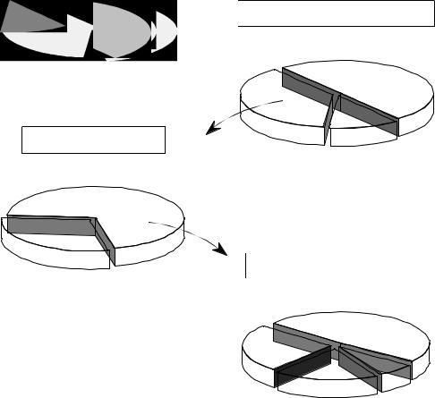
FIGURE 28-8
Major trends in DSPs. As illustrated in (a), about 38% of embedded designers have already switched from conventional microprocessors to DSPs, and another 49% are considering the change. In (b), about twice as many engineers use fixed point as use floating point DSPs. This is mainly driven by consumer products that must have low cost electronics, such as cellular telephones. However, as shown in (c), floating point is the fastest growing segment; over one-half of engineers currently using 16 bit devices plan to migrate to floating point DSPs
instance, suppose you are designing a medical imaging system, such a computed tomography scanner. Only a few hundred of the model will ever be sold, at a price of several hundred-thousand dollars each. For this application, the cost of the DSP is insignificant, but the performance is critical. In spite of the larger number of fixed point DSPs being used, the floating point market is the fastest growing segment. As shown in (c), over one-half of engineers using 16-bits devices plan to migrate to floating point at some time in the near future.
Before leaving this topic, we should reemphasize that floating point and fixed point usually use 32 bits and 16 bits, respectively, but not always. For
520 |
The Scientist and Engineer's Guide to Digital Signal Processing |
instance, the SHARC family can represent numbers in 32-bit fixed point, a mode that is common in digital audio applications. This makes the 232 quantization levels spaced uniformly over a relatively small range, say, between -1 and 1. In comparison, floating point notation places the 232 quantization levels logarithmically over a huge range, typically ±3.4×10 38. This gives 32-bit fixed point better precision, that is, the quantization error on any one sample will be lower. However, 32-bit floating point has a higher dynamic range, meaning there is a greater difference between the largest number and the smallest number that can be represented.
C versus Assembly
DSPs are programmed in the same languages as other scientific and engineering applications, usually assembly or C. Programs written in assembly can execute faster, while programs written in C are easier to develop and maintain. In traditional applications, such as programs run on personal computers and mainframes, C is almost always the first choice. If assembly is used at all, it is restricted to short subroutines that must run with the utmost speed. This is shown graphically in Fig. 28-9a; for every traditional programmer that works in assembly, there are approximately ten that use C.
However, DSP programs are different from traditional software tasks in two important respects. First, the programs are usually much shorter, say, onehundred lines versus ten-thousand lines. Second, the execution speed is often a critical part of the application. After all, that's why someone uses a DSP in the first place, for its blinding speed. These two factors motivate many software engineers to switch from C to assembly for programming Digital Signal Processors. This is illustrated in (b); nearly as many DSP programmers use assembly as use C.
Figure (c) takes this further by looking at the revenue produced by DSP products. For every dollar made with a DSP programmed in C, two dollars are made with a DSP programmed in assembly. The reason for this is simple; money is made by outperforming the competition. From a pure performance standpoint, such as execution speed and manufacturing cost, assembly almost always has the advantage over C. For instance, C code usually requires a larger memory than assembly, resulting in more expensive hardware. However, the DSP market is continually changing. As the market grows, manufacturers will respond by designing DSPs that are optimized for programming in C. For instance, C is much more efficient when there is a large, general purpose register set and a unified memory space. These future improvements will minimize the difference in execution time between C and assembly, and allow C to be used in more applications.
To better understand this decision between C and assembly, let's look at a typical DSP task programmed in each language. The example we will use is the calculation of the dot product of the two arrays, x [ ] and y [ ]. This is a simple mathematical operation, we multiply each coefficient in one
Chapter 28Digital Signal Processors |
521 |
a. Traditional Programmers
Assembly
C
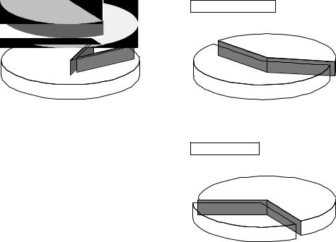
FIGURE 28-9
Programming in C versus assembly. As shown in (a), only about 10% of traditional programmers (such as those that work on personal computers and mainframes) use assembly. However, as illustrated in (b), assembly is much more common in Digital Signal Processors. This is because DSP programs must operate as fast as possible, and are usually quite short. Figure (c) shows that assembly is even more common in products that generate a high revenue.
b. DSP Programmers
Assembly
C
c. DSP Revenue
Assembly
C
array by the corresponding coefficient in the other array, and sum the products, i.e. x[0] × y[0] % x[1] × y[1] % x[2] × y[2] % þ. This should look very familiar; it is the fundamental operation in an FIR filter. That is, each sample in the output signal is found by multiplying stored samples from the input signal (in one array) by the filter coefficients (in the other array), and summing the products.
Table 28-2 shows how the dot product is calculated in a C program. In lines 001-004 we define the two arrays, x [ ] and y [ ], to be 20 elements long. We also define r e s u l t , the variable that holds the calculated dot
|
001 |
#define LEN 20 |
|
|
002 |
float dm x[LEN]; |
|
|
003 |
float pm y[LEN]; |
|
|
004 |
float result; |
|
TABLE 28-2 |
005 |
|
|
006 |
main() |
||
Dot product in C. This progam calculates |
|||
the dot product of two arrays, x[ ] and y[ ], |
007 |
|
|
and stores the result in the variable, result. |
008 |
{ |
|
|
009 |
int n; |
|
|
010 |
float s; |
|
|
011 |
for (n=0;n<LEN;n++) |
|
|
012 |
s += x[n]*y[n]; |
|
|
013 |
result = s |
|
|
014 |
} |
522 |
The Scientist and Engineer's Guide to Digital Signal Processing |
product at the completion of the program. Line 011 controls the 20 loops needed for the calculation, using the variable n as a loop counter. The only statement within the loop is line 012, which multiplies the corresponding coefficients from the two arrays, and adds the product to the accumulator variable, s. (If you are not familiar with C, the statement: s % ' x [n] ( y [n] means the same as: s ' s % x [n] ( y [n] ). After the loop, the value in the accumulator, s, is transferred to the output variable, result, in line 013.
A key advantage of using a high-level language (such as C, Fortran, or Basic) is that the programmer does not need to understand the architecture of the microprocessor being used; knowledge of the architecture is left to the compiler. For instance, this short C program uses several variables: n, s, result, plus the arrays: x [ ] and y [ ]. All of these variables must be assigned a "home" in hardware to keep track of their value. Depending on the microprocessor, these storage locations can be the general purpose data registers, locations in the main memory, or special registers dedicated to particular functions. However, the person writing a high-level program knows little or nothing about this memory management; this task has been delegated to the software engineer who wrote the compiler. The problem is, these two people have never met; they only communicate through a set of predefined rules. High-level languages are easier than assembly because you give half the work to someone else. However, they are less efficient because you aren't quite sure how the delegated work is being carried out.
In comparison, Table 28-3 shows the dot product program written in assembly for the SHARC DSP. The assembly language for the Analog Devices DSPs (both their 16 bit fixed-point and 32 bit SHARC devices) are known for their simple algebraic-like syntax. While we won't go through all the details, here is the general operation. Notice that everything relates to hardware; there are no abstract variables in this code, only data registers and memory locations.
Each semicolon represents a clock cycle. circular buffers in the main memory.
The arrays x [ ] and y [ ] are held in In lines 001 and 002, registers i4
001 |
i12 = _y; |
/* i12 points to beginning of y[ ] */ |
002 |
i4 = _x; |
/* i4 points to beginning of x[ ] */ |
003 |
|
|
004 |
lcntr = 20, do (pc,4) until lce; |
/* loop for the 20 array entries */ |
005 |
f2 = dm(i4,m6); |
/* load the x[ ] value into register f2 */ |
006 |
f4 = pm(i12,m14); |
/* load the y[ ] value into register f4 */ |
007 |
f8 = f2*f4; |
/* multiply the two values, store in f8 */ |
008 |
f12 = f8 + f12; |
/* add the product to the accumulator in f12 */ |
009 |
|
|
010 |
dm(_result) = f12; |
/* write the accumulator to memory */ |
TABLE 28-3
Dot product in assembly (unoptimized). This program calculates the dot product of the two arrays, x[ ] and y[ ], and stores the result in the variable, result. This is assembly code for the Analog Devices SHARC DSPs. See the text for details.